Nonlinear Waves

1. Intro
After the piece on Linear Waves, it only makes sense that I start this piece talking about Nonlinear Waves – from symmetry to asymmetry – from the processes of a zero residual to the complicacy of residuals. The nonlinearity is the characteristic signature of shallow water waves – and is also a recognizable feature of spectral wind waves that go through the nonlinear processes of interactions and high steepness. We have identified in earlier pieces that the single most important parameter, the Ursell Number, U = HL^2/d^3 (H is wave height, L is local wave length and d is local water depth) characterizes a wave as asymmetric or nonlinear, when U is greater than 5.0. The Ursell Number is universally applicable to all oscillatory flows, whether they are a short wave (like wind wave and swell) or a long wave (like tsunami, storm surge and tide).
Some of the materials covered in this piece on tidal nonlinearity are taken from my Ph.D. Dissertation (Dynamics of Coastal Circulation and Sediment Transport in the Coastal Ocean off the Ganges-Brahmaputra River Mouth, the University of South Carolina, 1992) along with two of my relevant publications:

• Suspended Sediment Movement in the Estuary of the Ganges-Brahmaputra-Meghna River System, Marine Geology, Elsevier, 1990.
• Suspended Sediment Distribution and Residual Transport in the Coastal Ocean off the Ganges-Brahmaputra River Mouth, Marine Geology, Elsevier, 1994.

Tsunami nonlinearity in Cnoidal and Solitary wave forms, before and at breaking is discussed in the Tsunami and Tsunami Forces piece on the SCIENCE & TECHNOLOGY page, therefore will not be repeated here.
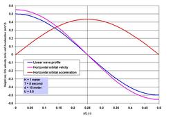
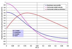
Many investigators are credited with developing the nonlinear wave theories. To name some, perhaps we can start with Stokes (British mathematician George Gabriel Stokes, 1819 – 1903; Stokes Finite Amplitude Wave Theory), J. S. Russell and J. McCowan (Solitary Wave Theory), D. J. Korteweg and D. de Vries (Cnoidal Wave Theory), Robert G. Dean (Stream Function Theory) and J. D. Fenton (Fourier Series Theory). Many more investigators were involved in expanding and refining the theories, some names include R. L. Weigel, L. Skjelbreia, R. A. Dalrymple and J. R. Chaplin.  
.  .  . 
2. Nonlinear Wave Kinematics
With this brief introduction, let us now try to understand what nonlinearity means exactly. To illustrate it, I have included two images showing the wave profile, surface horizontal orbital velocity and acceleration for the same 1 meter high 8 second wave, I have shown in the Linear Waves piece. Depicting the parameters for half the wave length, it is immediately clear how the crest is heightened and the trough is flattened when the wave propagates straight shoreward from U = 5.0 to 22.6 (note that 22.6 is near the threshold at which waves can also be treated as Cnoidal). Horizontal water particle velocity has nearly doubled at the crest with the reduction at the trough. For acceleration, the change is not only in the increase in magnitude but also in the phase shift from the symmetry at quarter wave length to the forward skewed distribution. Even this nonlinearity as complicated as it is – is a simplification of the reality because more processes such as reflection and interactions play a role in defining the wave evolution in the nearshore region.  
We have talked about Stokes Drift in the Transformation of Waves piece on the SCIENCE & TECHNOLOGY page. Stokes Drift or mass transport horizontal velocity represents a nonlinear residual in the direction of wave propagation, and is about one order less in magnitude than the horizontal orbital velocity. For the nonlinear wave at U = 22.6, while the peak surface horizontal orbital velocity is 0.96 meter per second, the drift is roughly about 5 centimeter per second. This drift may seem very small, but a particle traveling at this speed will travel to 180 meter in an hour.   
Before going further, an important parameter – the local wave length L needs some attention. We have seen in the Linear Waves piece that determining L iteratively has become easy with the modern computing systems, or by applying the Hunt (H. N. Hunt, 1979) method. However as waves become nonlinear, the wave length starts to deviate from the L determined by Linear Wave Theory. It turns out that at U > 5.0, the deviation becomes increasingly larger as U increases, but remains within about 10%.    
Why understanding the nonlinear wave phenomenon is important? A simple answer to the question is that the nonlinearity of oscillatory flows is responsible for many processes that define a coastal system behavior and characteristics, and in the behaviors of hydrodynamic loading on, and stability of in-water and waterfront structures. Let me try to outline three of them briefly.
.  .  .
3. Consequences of Wave Asymmetry and Nonlinearity
The first is the effects of the increase and phase-shift of the orbital velocity and acceleration as shown in the images. These processes have significant implications for wave-induced drag, lift and inertial Morison forces (J. R. Morison and others, 1950; forces on slender members) on coastal and port structures. Horizontal drag and inertial forces are relevant in terms of the maximums; therefore as the maximums increase so do the forces. The pieces Characterizing Wave Asymmetry and Wave Forces on Slender Structures discusses such aspects.
When I stated about the phase-shifts and the relevance of maximums, did anyone notice a contradiction in my statement of Morison forces? Well there is one – the contradiction is due to one of the methods engineers often apply to accommodate some maximums – however unscientific the method may appear – for a conservative and safe design by implanting the so-called Hidden Factor of Safety. Let us discuss more of this aspect in the SCIENCE & TECHNOLOGY page along with my ISOPE paper (Wave Loads on Piles – Spectral Versus Monochromatic Approach, 2008).
How does one define the increased nonlinear maximums in terms of asymmetry? Some of my works (not published) indicate that one could relate the amplitude asymmetry of velocity and acceleration in terms of U. Once such a relation is established, it becomes rather easy to determine the nonlinear Morison forces.    
The second is the effect of the nonlinearity as it interacts with the seabed – the processes generate enhanced turbulence, and when the threshold is exceeded, they are responsible for erosion and resuspension of sediments. Depending on circumstances, nonlinearity is responsible for residual transports toward the onshore, offshore or longshore directions. How to characterize the residuals? I will try to answer this question based on my Ph.D. works and the two relevant publications already mentioned. This will be done for tide, tidal currents and Suspended Sediment (mostly fine sediments that are kept in suspension in the water column by currents and turbulence) Concentrations (SSC).
One method to indicate the residuals e.g. of to-and-fro tidal currents (currents are vector kinematics with both magnitude and direction) is to make vector addition of the individual measurements (such as hourly) – such a method immediately shows that a circle cannot be completed because of nonlinearity – and also due to the effects of other superimposed currents such as a river discharge or wind drift, if present. If seaward currents are high at river mouths, residuals are mostly seaward; on the other hand, in absence of a river current or wind drift, tidal asymmetry is responsible for landward transport, and accumulation of fine sediments in tidal flats. These effects of varying superimposed currents and asymmetries often stratify a shallow and wide coastal system horizontally – the coastal ocean off the Ganges-Brahmaputra system is one of such systems. The residual current vectors are a good indicator of, and to where suspended fine (mostly silt and clay sized particles) sediments or water-borne contaminants are likely to end up.
The combined tidal current and SSC measurements over time and over the depth can be analyzed applying a procedure known as the linear perturbation principle – a method of vector averaging and identifications of perturbations from the mean. The procedure yields some 5 terms accounting for non-tidal actions, and for the asymmetries of tide, tidal currents and the hysteresis of SSC over time and over the depth. Such methods of separating the components are very useful to provide valuable insights into the identification of processes responsible for certain actions and behaviors.
The third is on the most dynamic region of wave action – the surf zone. This is the region where the wave nonlinearity reaches its ultimate stage by breaking as the horizontal wave orbital velocity overtakes the celerity. The breaker line or rather the breaker zone is not fixed, because the breaking depth together with the effects of rising and falling tides is related to the changing wave height. The transformation of the near-oscillatory waves into the near-translatory water motion by wave breaking and energy dissipation is the most recognizable process in this zone. Let us try to see more of it at some other time.

.  .  .  .  .

- by Dr. Dilip K. Barua, 20 October 2016