Science and technology
working with nature- civil and hydraulic engineering to aspects of real world problems in water and at the waterfront - within coastal environments
 This piece is a continuation of the Sea Level Rise – the Science post on the Nature page. Let us attempt to see in this piece how different thoughts are taking shape to face the reality of the consequences of sea level rise (SLR). The consequences are expected across the board – in both biotic and abiotic systems. But to limit this blog to a manageable level, I will try to focus – in an engineering sense – on some aspects of human livelihood in frontal coastal areas – some of the problems and the potential ways to adapt to the consequences of SLR (In a later article Warming Climate and Entropy, posted in December 2019 – I have tried to throw some lights on the climate change processes of the interactive Fluid, Solid and Life Systems on Earth – the past, the present and the future).
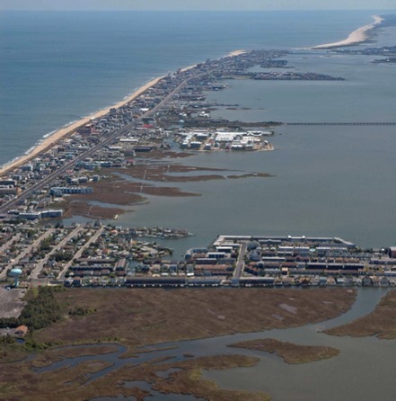
Before doing that let us revisit one more time to point out that all familiar lives and plants have a narrow threshold of environmental and climatic factors, within which they can function and survive. This is in contrast to many microorganisms like Tardigrades, which can function and survive within a wide variation of factors. Therefore adaptation can be very painful, even fatal when stresses exceed the thresholds quickly – in time-scales shorter than the natural adaptation time. . . . What is stress? Global warming and SLR literature use this term quite often. Stress is part of the universal cause-effect, force-response, action-reaction, stress-consequence duo. In simple terms and in context of this piece, global warming is the stress with SLR as the consequence – in turn SLR is the stress with the consequences on human livelihood in the coastal zone. Again, as I have mentioned in the previous piece, the topic is very popular and literature are plentiful with discussions and opinions. The main resources consulted for this piece are the adaptation and mitigation chapters of the reports worked on by: UN entity IPCC (Intergovernmental Panel on Climate Change), US NOAA (National Oceanic and Atmospheric Administration), and USACE (United States Army Corps of Engineers). Before going further, it will be helpful to clarify the general meanings of some of the commonly used terms – these terms are used in contexts of system responses and reactions – susceptibility, prevention, the ability to adjust to changes, and the ability to cope with repeated disruptions. The first is vulnerability – the susceptibility and inability of a system to cope with adverse consequences or impacts. One can simply cite an example that human habitation, coastal and port infrastructure in low lying areas are more vulnerable to SLR than those lying in elevated areas – and so are the developing societies than the developed ones. The second is known as mitigation – the process of reducing the stresses to limit their impacts or consequences. We have seen in the NATURE page that there could be some 8 factors responsible for SLR. But scientists have identified that the present accelerated SLR is due to the continuing global warming caused by increased concentration of greenhouse gases. This anthropogenic factor is in human hands to control; therefore reducing greenhouse gases is one of the mitigation measures. The third is adaptation – the process of adjusting to the consequences of expected or imposed stresses, in order to either lessen or avoid harm, or to exploit beneficial opportunities. This is the primary topic of this piece – how humans could adjust to the consequences of SLR. The fourth is closely related to adaptation and is known as resilience – the ability to cope with repeated disruptions. It is not difficult to understand that adaptation process can become meaningless without resilience. Also to note that a successful mitigation can only work with some sort of adaptation – for example, adaptation by innovating new technologies to control and limit greenhouse gas emission. However, one may often require to compromise or make trade-offs between mitigation and adaptation processes to chalk out an acceptable solution. . . . I have included an image (credit: anon) of human habitation and township developed on a low lying barrier island. Similar developments occur in most coastal countries – some are due to the pressure of population increase, while others are due to the lack of foresight and understanding by regulating authorities. Such an image is important to look at, to reflect on and to think about human vulnerability, and the processes of mitigation, adaptation and resilience to the consequences of SLR. A series of ASCE Collaborate discussions gives a glimpse of SLR on low-lying airports. Before going further, some aspects of climate change that exacerbate the SLR effects need to be highlighted. The first is the enhanced wave activity associated with SLR. We all have seen the changing nature of waves sitting on a shoreline during an unchanging weather condition – less wave activity at low tide and enhanced waves as tide rises. Why does that happen? One reason is the depth-limited filtering of wave actions – for a certain depth only waves smaller than about 4/5th of water depth could pass on to the shore without breaking. Therefore, as the water level rises with SLR, the numbers of waves propagating on to the shore increase. The second is the enhanced storminess caused by global warming. All the climate change studies indicate the likelihood of increase in storminess both in intensity and frequency – and perhaps we are witnessing symptoms of that already. High wind storms are accompanied by high storm surges and waves together with torrential rainfall and terrestrial flooding. . . . What are the consequences of SLR? The consequences are many – some may not even be obvious at the present stage of understanding. They range from transgression of sea into the land by erosion, inundation and backwater effect, to salt-water intrusion, to increased forces on and overtopping of coastal waterfront structures. If the 2.0 meter SLR really (?) happens by the end of the 21st century, then it is impossible for one not to get scared. I have included a question mark to the 2.0 meter SLR because of the high level of uncertainty in the predictions by different organizations (see the Sea Level Rise – the Science blog on the NATURE page). For such a scenario, the effective SLR is likely to be no less than 10.0 meter affecting some 0.5 billion coastal population. The effective SLR is an indication of the range of consequences that a mean SLR would usher in. Let me try to provide a brief outline of the consequences. First, one should understand that the transgression of sea into the land is not like the invasion by a carpet of water gradually encroaching and inundating the land. It is rather the incremental incidences of high-tide-flooding combined with high wave activity. The result is the gradual net loss of land into the sea through erosion and scour, sediment-morphological readjustments and subsequent submergence. . . . What adaptation to SLR really means? Let us think of coastal population first. Survival instinct will lead people to abandon what they have, salvage what they can, and retreat and relocate themselves somewhere not affected by SLR. Although some may venture to live with water around if technological innovations come up with proven and viable measures. There are many traditional human habitations in seasonally flooded low lands, and also examples of boathouses around the world. Therefore, people’s lives are not so much at stake in direct terms; it is rather the monetary and emotional losses they would incur – losses of land, home and all of their valuable assets and memories. This adaptation process will not be equally felt by all the affected people. Rich people and perhaps many in developed societies are likely to cope with the problem better than the others. Perhaps the crux of the problem will be with civil infrastructure. One can identify them as four major types:
Some other aspects of the problem lie with the intrusion of sea saline water into estuaries, inlets and aquifers. Coastal manufacturing and energy facilities requiring freshwater cooling will require adapting to the SLR consequences. The problem will also be faced with the increased corrosion of structural members. . . . What to do with this huge problem of the existing civil infrastructure? What does adaptation mean for such a problem? One may think of renovation and reinforcement, but the likelihood of success of such an adaptive approach may be highly remote. How do the problems translate to the local and state’s economy? What about abandoning them to form submersed reef – declaring them as Water Park or sanctuary? - leaving many as remnants for posterity like the lost city of Plato’s (Greek Philosopher, 423 – 347 BCE) Atlantis? There are no easy answers to any of these questions; but there is no doubt that stakes are very high. We can only hope that such scenarios would not happen. What is important and is being initiated across the board is the formulation of mitigation and adaptation strategies and policies. Such decision making processes rely on the paradigm of risk minimization – but can only be meaningful if uncertainties associated with SLR predictions are also minimized. One important area of work where urgent attention is being paid is in the process of updating and redefining the standards, criteria and regulations required for robust planning and design of new coastal civil infrastructure. However, because of uncertainties in SLR predictions even this process becomes cumbersome. Placing concrete and steel to build anywhere is easy, what is not easy is envisioning the implications and the future. . . . Apart from the 2017 NAP Proceedings – 24847 Responding to the Threat of Sea Level Rise, the 2010 publication – 12783 Adapting to the Impacts of Climate Change is an excellent read on possible options – as approaches to adapt to different stresses and consequences imposed by climate change. Well, some thoughts in a nutshell, shall we say? But mitigation of and adaptation to a complex phenomenon like global warming, climate change and SLR must be understood as an evolving process – perfection will only likely to occur as things move forward. And one should not forget that the SLR problems as complex and intimidating as they are, are slow in human terms – therefore the adaptation processes should be conceived in generational terms, but all indications suggest that the thinking and processes must start without delay. Fortunately all members of the public are aware of the problem and are rightly concerned - whether or not things are rolling in the right direction. Hopefully, this will propel leaders to take thoughtful actions. . . . Here is an anecdote to ponder: The disciple said, “Sir, adaptation is a very strong word perhaps more than what we think it is.” The master replied, “Yes, it does have a deeper meaning. One is in the transformation of the personalities undergoing the adaptation processes. It is a slow and sequential process ensuring the fluidity of Nature and society and evolution. If one thinks about the modern age of information, travel and immigration, the process is becoming much more encompassing – perhaps more than we are aware of. But while slow adaptation is part of the natural process, the necessity of quick adaptation can be very painful and costly.” . . . . . - by Dr. Dilip K. Barua, 29 September 2016
0 Comments
 With this piece I am breaking my usual 3-3-3 cycle of posting the blogs on the NATURE, SOCIAL INTERACTIONS and SCIENCE & TECHNOLOGY pages. The reason is partly due to the comment of one of my friends who said, it is nice reading the Nature and Science & Technology pages. Hope you would share more of your other experiences in theses pages. Well, I have wanted to that but in the disciplined order of 3-3-3 postings. But this does not mean that the practice cannot be changed to concentrate more on the technical pages. Let us see how things go – a professional experience spanning well over 3 decades is long enough to accumulate many diverse and versatile humps and bumps, distinctions and recognitions, and smiles and sadness.
. . . This piece can be very long, but I will try to limit it to the usual 4 to 5 pages starting from where I left – some of the model basics described in the Natural Equilibrium blog on the NATURE page, and in the Common Sense Hydraulics blog on this page. To suit the interests of general members of the public, I will mainly focus on the practical aspects of water modeling rather than on numerical aspects. A Collaborate-ASCE discussion link highlights aspects of water modeling validation issues. The title of this piece could have been different – numerical modeling, computational modeling, hydrodynamic modeling, wave modeling, sediment transport modeling, morphological modeling . . . Each of these terms conveys only a portion of the message what a modeling of Natural water means. The Natural waters in a coastal environment are 3-dimensional – in length, width and depth, subjected to the major forces – externally by tide and wave at the open boundaries, wind forcing at the water surface and frictional resistance at the bottom. The bottom can be highly mobile like in alluvial beds, or can be relatively fixed like in a fjord. Apart from these regular forcings coastal waters are also subjected to extreme episodes of storm surge and tsunami. A model generally refers to a collective term for: ‘representations of essential system aspects, with knowledge being presented in a workable form.’ (Delft Hydraulics 1999). A system refers to: ‘A system is a part of reality (isolated from the rest) consisting of entities with their mutual relations (processes) and a limited number of relations with the reality outside of the system.’ A model, therefore, is the representation of a system if it describes the structure of the system-entities and relations. Models can be depicted in all different kinds of presentations: ordinary languages, schematics, figures, mathematics, etc. A mathematical model describing the relations in terms of independent and dependent variables is the mathematical translation of a conceptual model. Non-mathematical representation of system aspects is known as the conceptual model. A schematic of different hydraulic models and relevant understandings is presented in the image. This image is taken from my draft lecture note – prepared for the students, while teaching at the Florida Institute of Technology. . . . While the Natural coastal setting is 3-dimensional, it is not always necessary to treat the system as such in a model. Depending on the purpose and availability of appropriate data, coastal systems can be approximated as 2-dimensional or 1-dimensional. The 2-dimensional shallow-water approximation is possible especially when the aspect ratio (depth/width) is low. When a channel is very long and the aspect ratio is relatively high, it can even be modeled as 1-dimensional. Apart from these dimensional approximations, some other approximations are also possible because all terms of the governing equations do not carry equal weight. I have tried to highlight how to examine the importance of different terms in a conference presentation (A Dynamic Approach to Characterize a Coastal System for Computational Modeling and Engineering. Canadian Coastal Zone Conference, UBC, 2008). The technique known as scale analysis lets one to examine a complicated partial differential equation by turning it into a discrete scale-value-equation. My presentation showing the beauty of scale analysis is highlighted for the governing hydrodynamics of fluid motion – the Navier-Stokes Equation (Claude-Louis Navier, 1785 – 1836 and George Gabriel Stokes, 1819 – 1903). It was further demonstrated in my Encyclopedia article, Seabed Roughness of Coastal Waters for practical workable solutions. The technique can also be applied for any other equation – such as the integral or phase-averaged wave action equation, and the phase resolving wave agitation equation. Many investigators deserve credit for developing the phase-averaged wave model – which is based on balancing the wave energy-action. The phase-resolving wave model is based on the formulation by Boussinesq – the French mathematician and physicist Joseph Valentin Boussinesq (1842 – 1929). The latter is very useful in shallow-water wave motions associated with non-linearity and breaking, and in harbors responding to wave excitation at its entrance. . . . A Power Point presentation of model-simulated south-bound longshore currents that could develop during an obliquely incident storm wave from the northeast is shown in Littoral Shoreline Change in the Presence of Hardbottom – Approaches, Constraints and Integrated Modeling. This title was presented at the 22nd Annual National Conference on Beach Preservation Technology, St. Pete Beach, Florida, 2009 on behalf of Coastal Tech. The incident wave is about 4 meter high generated by a Hurricane Frances (September 5th 2004) like storm on the Indian River County shores in Florida. . . . Water modeling is fundamentally different and perhaps more complex – for example, from structural stability and strength modeling and computations. This assertion is true in a sense that a water model first aims to simulate the dynamics of Natural flows to a reasonable level of acceptance, before more can be done with the model – to use it as a soft tool to forecast future scenarios, or to predict changes and effects when engineering interventions are planned. Water modeling is like a piece of science and art, where one can have a synoptic view of water level, current, wave and sediment transport, and bed morphology within the space of the model domain simultaneously – this convenience cannot be afforded by any other means. If the model results are animated, one can see how the system parameters evolve in response to forces and actions – this type of visuals is rather easy and instructive for anyone to understand the beauty and dynamics of fluid motion. For modelers, the displays elevate his or her intuition helping to identify modeling problems and solutions. . . . Before going further, I would like to clarify the two terms I have introduced in the Coastal River Delta blog on the NATURE page. These two terms are behavioral model and process-based model. Let me try to explain the meaning of these two terms briefly by illustrating two simple examples. The simple example of a behavioral model is the Bruun Rule or the so-called equilibrium 2/3rd beach profile, proposed by Per Bruun in 1954 and refined further by Bob Dean (Robert G. Dean, 1931 – 2015) in 1977. The relation simply describes a planer (no presence of beach bars) beach depth as the 2/3rd power of cross-shore distance – without using any beach-process parameters such as the wave height and wave period. The only other parameter the Rule uses is the sand particle settling velocity. This type of easy-to-understand behavioral models that does not look into the processes exciting the system, exists in many science and engineering applications. The behavioral models capture response behaviors that are often adequate to describe a particular situation – however they cannot be applied or need to be updated if the situation changes. The simple example of a process-based model is the Chezy Equation (Antoine Chezy, 1718 – 1798) of the uniform non-accelerating flow – that turns out to have resulted from balancing the pressure-gradient force against the frictional resistance force. In this relation velocity of flow is related to water depth, water level slope (or energy slope) and a frictional coefficient. The advantage of a process-based model is that it can be applied in different situations, albeit as an approximation in which it has been derived. . . . Let us now turn our attention to the core material of this piece – the numerical water modeling. The aspects of the scale modeling used to reproduce water motion in a miniature replica of the actual prototype in controlled laboratory conditions are not covered in this piece. These types of models are based on scale laws by ensuring that the governing dimensionless numbers are preserved in the model as in the prototype. I have touched upon a little bit of this aspect in the Common Sense Hydraulics piece on this page. I have been introduced to programming and to the fundamentals of numerical water modeling in the academic programs at IHE-UNESCO and at the USC. My professional experience started at the Land Reclamation Project (LRP) with the supports from my Dutch colleagues and participating in the hydrodynamic modeling efforts of LRP. Starting with programmable calculators, I was able to develop several hydraulic processing programs and tools – later translating them to personal computer versions. I must say, however that my knowledge and experience have really taken-off and matured during my heavy involvement with numerical modeling efforts in several projects in Canada, USA and overseas. This started with a model selection study I conducted with UBC for the Fraser River in British Columbia. A little brief on my modeling experiences. They include the systems: 8 in British Columbia (e.g. 2006 Coastal Engineering Tsunami paper), 1 in Quebec, 1 in Newfoundland and Labrador, 2 in Florida, 1 in Texas and 1 in Virginia (ASCE Ports 2013 Inlet Sedimentation paper). Among the modeled processes were hydrodynamics, wave energy actions, wave agitations, coupled wave-hydrodynamics, and coupled-wave-hydrodynamics-sediment transport-morphologies. The model forcings were tide, wind and wave, storm surge and tsunami. I will try to get back to some of the published works at some other time. Perhaps it is worthwhile to mention here that modeling experience is also a learning exercise; therefore one can say that all hydraulic engineers should have some modeling hand-on experiences, because they let him or her to acquire very valuable insights on hydraulics – simply using available relations to compute forces and parameters may prove incomplete and inadequate. . . . In the Uncertainty and Risk piece on this page, some unavoidable limitations and constraints of models are discussed. Let me try to outline them in some more details. Model uncertainties can result from 8 different sources:
. . . Before a model is ready for application, it requires going through a process of validation. This process of comparing model outputs against corresponding measurements leads to tuning and tweaking of parameters to arrive at acceptable agreements. It is also reinforced with sensitivity analysis to better understand the model responses to parameter changes. A National Academies Publication discusses some important steps on model verification and validation. In Natural Equilibrium piece – here are what outlined: For modelers, the challenges are to translate the continuum of space and time into the discretized domain of a model – such as: what to include, what to leave out, what to smooth out, and what are the consequences for such actions. How best to take account of practical constraints and describe forcing at the boundaries to be realistic but at the same time avoiding model instability. Reactive forces like frictional resistance are notoriously non-linear – therefore it is important to watch how parameterization of these forces affects results. Let us attempt to understand this crucial steps by proposing an acronym: MRCAP – Model-Reality Conformity Assurance Processes . . . Model-Reality Conformity Assurance Processes (MRCAP) The conformity of a model with the reality of interest is an important issue – not only for computational modeling – but also for any sort of modeling – including scale modeling. Large civil engineering practices and projects – especially its open-water hydraulic engineering tenet – are highly dependent on both of these modeling efforts. Scale modeling is continuously getting marginalized because of its cost – also, because of the growing robustness of and confidence in numerical models. Models are a replicating tool of a certain physical reality. Like with developing any tool – and before being assured as a validated product – they need experimentation, refinement and calibration to satisfy the governing laws and equations. Yet, models are a soft tool that accompany uncertainties of different sorts. But, the same is true with any physical reality – the quantitative nature of which can only be understood through measurements or sampling (more in Uncertainty and Risk). I like to begin explaining this interest aspect of water modeling with the help of MRCAP – Model-Reality Conformity Assurance Processes. The purpose of MRCAP is to produce a credible or conformal simulation of the reality. This reality can either be the system of as is existing conditions, or in combination with the envisioned scenarios of engineering installations. The latter is to examine and determine the forces on and effects of such interventions. An engineer’s computational modeling interest lies in both of them – and in the context of this article – in computational modeling of waters. At least four reference materials must be cited while explaining MRCAP. The first is the 1998 document (The Guide for the Verification and Validation of Computational Fluid Dynamics Simulations, AIAA Guide 1998). Many subsequent publications on this interesting topic trace their roots to this guide. They include: Oberkampf et al (Verification and Validation for Modeling and Simulation in Computational Science and Engineering Applications 2002); ASME 2020 (Standard for Verification and Validation in Computational Solid Mechanics); and the 2024 NAP Publication # 27747 (Quality Processes for Bridge Analysis Models). They provide the essence of a broad MRCAP framework. These reference materials shows MRCAP as consisting of three processes – starting with qualification, to verification and validation. The emphasis on these three processes form a loop of three end points: Reality ↔ Mathematical Model ↔ Computational Model ↔ Reality. The iterative processes between the first two was termed as ‘Model Qualification’. In 1979, the Society for Computer Simulation defined it as: “Determination of adequacy of the conceptual model to provide an acceptable level of agreement for the domain of intended application.” The term ‘conceptual model’ has been replaced by mathematical model in later evolution of definitions. Here is something from Natural Equilibrium: The workable form of a model can be concepts, ordinary language, schematics, figures and mathematics. A conceptual model is a non-mathematical representation of the inter-relationship of system elements. A mathematical model is the translation of a conceptual model in mathematical terms of variables and numbers. This step essentially indicates processes of examining and re-examining the Representitiveness of the selected mathematical model with reality. The degree of representitiveness is the first of the 8 model uncertainties. Next, the iterative processes between the selected mathematical model and the implemented computational model was termed as ‘Verification’. In ASME wording, verification is: “the process of determining that a computational model accurately represents the underlying mathematical model and its solution”. Among the 8 sources of uncertainties, the degree of Empiricism, Discretization of the Continuum, Iteration to Convergence, Rounding-Off and Numerical Code tells to what extent the verification processes are successful. The first four sources of uncertainties are listed as 2 – 5, the last one is listed 8. ‘Validation’ processes comprise the final step connecting the Computational Model with Reality. The degree of the rest two sources of uncertainty, 6 and 7, Application and Modeler determine how validation processes are successful. Again, in ASME wording validation is: “the process of determining the degree to which the model is an accurate representation of corresponding physical experiments from the perspective of the intended uses of the model” In the broad framework of modeling terminology – the AIAA guide emphasizing verification and validation is known as V&V. . . . Model Performance The V&V framework misses something very important – at least from computational water modeling perspective of model performance. This something is known as ‘Calibration’ – a crucial step. Calibration is an iterative process where a modeler tweaks terms and parameters to tune and fine-tune a computational model. Also, the modeler uses the term verification in a different sense than what is described the AIAA guide. To avoid confusion, let us term it as ‘Model Results Verification’ This step is an essential confidence building exercise of MRCAP – and is done by simulating a scenario – that is different in time and space than the calibration scenarios. It is important to understand these aspects further. Let me begin with a short introduction – focusing primarily on Coastal Water Modeling. Wave, hydrodynamic and sediment transport computational modeling activities occupy a significant portion of analysis in coastal engineering, and form an integral component of complex and large projects. Although interchangeably used, a distinction has to be made between the terms known as numerical and computational modeling. While numerical modeling mainly deals with transforming complex differential equations describing the physics – into algebraic equations and to numerical codes; computational modeling is the art of transforming a physical problem to the computational domain of a numerical model and executing simulations to replicate the physics. The fundamental to all these efforts is the use of a computer which cannot handle complex differential equations, but can work with numbers generated by algebraic equations and codes to perform these operations. A person can either be a numerical modeler, a computational modeler or both. In the past, there was no such distinction, but this is becoming more evident as modeling efforts continue to proliferate and expand – with the availability of many commercial modeling software suites. The rationale for calibration, and model results verification can be appreciated from the requirements expected of modelers. They must understand: (1) the theory of physics being modeled; (2) the basics of numerical modeling formulation; (3) the computational methods of the model being applied; (4) the processes describing the area of application including initial and boundary conditions; (5) dynamic coupling of wave, hydrodynamics, and sediment transport-morphology, if applicable; (6) the wave and hydrodynamic interactions with structures, if present; (7) uncertainties present both in measurements and model outputs; (8) tuning of model parameters by calibration and verification; (9) interpretation of model outputs to the tune of conformity assurance; (10) last, but not the least, the pre- and post-processing of computational inputs and outputs. In my 2009 FSBPA Power Point Presentation (Barua, Walther, Triutt; 2009. Littoral Shoreline Change in the Presence of Hard Bottom – Approaches, Constraints and Integrated Modeling), I have tried to shed light on two aspects of model uncertainties and constraints – resulting primarily from model data sources. In most cases of coastal water computational modeling – modelers have to deal with and use data available from regional sources – the quality of them – are really not known. In addition, quantity, resolution and frequency of such available data are mostly inadequate. These constraints impose limitations on the modeler’s efforts to calibrate and verify the model. This can be compared with the site-specific dedicated measurements campaign for large projects – where a modeler has control on measurement quantity, quality, resolution and frequency. . . . Finally, a few words on the rationale of such requirements, and on the statistical assessments of model performance – leading to the soundness of MRCAP. The rationale for calibration and verification can best be understood by recognizing the various elements and terms of the governing equations – that are complete with the actions of some reactive forces (referred to as closure terms in early literature). In hydrodynamic equations the reactive forces appear as solid boundary roughness and fluid-flow turbulence – nature of turbulence. These forces are parameterized in the governing equations – therefore, can be tweaked to attain an equilibrium of forces ↔ responses. The processes also include various levels of sensitivity analyses. A few statistical assessments are made comparing model results with relevant measurements. They include: Mean Absolute Error (MAE), Root Mean Square Error (RMSE), Brier Skill Score (BSS; or Assessment BSA). When MAE is divided by the average of the measured parameter, it turns into RMAE. A modeler goes through the iterative processes of calibration and verification to minimize MAE, RMSE or RMAE errors, while trying to maximize BSS. Use of statistics is an attempt to smooth out disagreements assuming that for a certain value of the statistical parameter – the model performance is acceptable. According to the suggestions by Van Rijn et al (2003) the good criteria are indicated by the following: 0.05 < RMAE of wave height < 0.1; 0.1 < RMAE of velocity < 0.3; 0.6 < BSS of bed level change <0.8. . . . I have often been asked whether water modeling is worth the efforts and costs. My univocal answer to the question is yes. In this age of quickly improving digital computations, displays, animations and automations, it would be a shame if one thinks otherwise. Science and engineering are not standing still – the capability of numerical models is continually being refined and improved at par with the developments of new techniques in the computing powers of digital machines. Like all project phases, a water model can be developed in phases – for example, starting with a course and rough model with the known regional data. Such a preliminary model developed by experienced modelers can be useful to develop project concepts and pre-feasibilities, and can also help planning measurements for a refined model required at subsequent project phases. We have tried to conclude that a model is a soft tool; therefore its performance in simulation and prediction is not expected to be exact. This means that one should be cautious not to oversell or over-interpret what a model cannot do. But even if a water model is not accurate enough to be applied as a quantitative tool, it can still be useful for qualitative and conceptual understandings of fluid motion, in particular as a tool to examine the effectiveness and effects of engineering measures under different scenarios. . . . Here is an anecdote to ponder: The disciple asked the master, “Sir, what does digitization mean to social fluidity or continuity?” The master replied, “Umm! Imagine a digital image built by many tiny pixels to create the totality of it. Each of these pixels is different, yet represents an essential building block of the image puzzle. Now think of the social energy – the energy of the harmonic composite can similarly be high and productive when each building block has the supporting integrity and strength.” . . . . . - by Dr. Dilip K. Barua, 22 September 2016 |
 RSS Feed
