Science and technology
working with nature- civil and hydraulic engineering to aspects of real world problems in water and at the waterfront - within coastal environments
 Given a mechanical civilisation the process of invention and improvement will always continue, but the tendency of capitalism is to slow it down, because under capitalism any invention that does not promise fairly immediate profits are suppressed. This saying of George Orwell (1903 – 1950) touches upon some very important issues associated with industrialization (mechanical civilisation) and capitalism. They are – the potential for unstoppable forward march of industrialization and some inhibitive effects of capitalism on it. In modern understanding, capitalism is an immediate profit making system in which the investor of the capital (primarily meant to be private) owns the enterprise – utilizing the services of machines and human labor. The human labor force that contributes to building up the capital - is not entitled to claim any share of the enhanced capital - it is only the executives who can claim so - the reward to them comes in the guise of shares, generous contract packages and hefty bonuses.
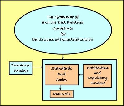
The general principle of capitalism – perhaps without so much forceful emphasis on immediate profit making – is the earliest form of doing trades and commerce in human history. In earlier times, in all cultures ideas like harmony (some terms like sustainability were not vogue then) and symmetry were thought important for a healthy society (although one can argue whether such a healthy society was ever achieved). But as we shall see later, the 18th century definition of capitalist economy by Adam Smith (1727 – 1790) – twisted this term giving it a meaning that gave impetus to myopic view, shortsightedness and selfishness – stoking mistrusts and animosity among individuals – with all the meandering outbursts of f-word, flash anger and cursing associated with them. A 20th century American economist – Milton Friedman (1912 – 2006) gave further boost to Adam Smith’s theory by proposing the so-called Friedman Doctrine in 1970. It says . . . there is one and only one social responsibility of business – to use its resources and engage in activities designed to increase its profits . . . He further stressed that businessmen with a social conscience . . . are unwitting puppets of the intellectual forces that have been undermining the basis of a free society . . . In this doctrine the definition of social responsibility is twisted – in order to justify the triumphant victory of money-making freedom. With such definitions that reinforced the forces of modern capitalism – the vicious dog-eat-dog-world is unleashed – and turned governing democracy into capitocracy. In recent times with the unregulated and unguarded internet dependent communications and activities (see Artificial Intelligence - the Tool of No Limit) - the works of bad actors - have only been proliferating many times. Realizing the importance of the capitalist context of industrialization – let us attempt to delve further into it in simple terms – through the lens of critical thinking, so to say – because it is necessary to orient ourselves to the true perspectives associated with this topic. . . . First, it is interesting to note that the immediate profit making – fits right into a democratic politician’s narrative – because his or her political lifetime and thinking revolves around short time scales from one election to another. One may, therefore infer that modern democracy – representing nothing more than party dictatorships rotating every few years – is perhaps the right tool to promote capitalism – because politicians can brag and campaign about how many material gains (even the bad ones – that become apparent in later times - and are gained at the expense of tax-payers) they made during their tenure. Further, the philosophy of large international financial institutions like IMF and World Bank also fits right into this paradigm – because they press and put conditions on poor countries (who appeal for help to ride over difficult times and alleviate debt servicing) to minimize costs for immediate profit making – by cutting wages and benefits to the hard working labor force, or sell state-owned enterprises to private ownerships. The rationale of Orwell observation can simply be outlined like this. Some industrialization processes of innovative and humane nature (such as extensive basic research; scientific exploration; nature, wildlife and environment protection, public welfare and health care; etc) that do not promise immediate profit (in monetary terms, but profits in terms of longterm benefits and others do accumulate) – largely remain outside the interest areas of capitalist enterprises. It also says why a capitalist system pampers majority (having an eye on large consumer base and labor force) – ethnic, religious or otherwise – by downplaying and ignoring the equal rights for minorities - more so for minority of minorities. Although governing principles of any country spell out equality in paper. Or, why some communities brag about or campaign for demographic changes in their favor – to implant longterm changes in a society. His observation also implies – why significant impact making individuals – the discoveries they make in the innovative efforts of laying out enlightened scientific principles, methods, ideas, and philosophies – remain poor and unappreciated during their lifetime. The selfish capitalist societies, however do not hesitate to profit from their discoveries at a later time. The observation further indicates that in smaller economies, industrialization may struggle to take-off because in such economies it is difficult to ensure immediate return of investments; or even in large economies where conditions are too stringent to function smoothly. However nowadays, governmental grants, guarantees, tax-incentives and bailout promise are attracting private capitals to venture in (one such area being the gov-private partnership). It is not difficult to see that the burden of all these gov initiatives falls ultimately on the shoulders of general public – with the gov levying taxes and gradually impoverishing people to make gov-private capitals fat and successful. In a capitalist system power is bestowed upon the owner of material wealth (money, to be exact) – and everyone else is a labor – irrespective of who they claim to be – whether white or blue color (although top white-color executives are treated as an associate and shareholder, while the lower white colors and blue-colors remain voiceless servants). Everything else – the immaterial wealth (such as happiness, see Happiness), is considered unimportant and therefore is taken out of the equation, or takes back seat. In such societies, the governing seats of power must withhold and promote the proliferation of private capital by assisting to find new markets for industrial goods and services. While such actions are incumbent upon the gov to assure the security of capital growth and flow – it does not and is reluctant to take any initiative or responsibility to assure job security to the labor force. However, the movement for organized labor force has paved a way - and Labor Unions are allowed in most countries. But, the capitalist outfit has its hand on it as well by imposing legal restrictions - in the manners of who and where such unions can be organized. Thus, another asymmetric system is imposed to allow a small fraction of the labor force the privilege of collective bargain power - while most are left out of the loop. Here, the rules of business take precedence over principles (as Dr BR Ambedkar, 1891-1956, outlined it, see The Mahatma – a Tribute). Further, to hide wealth distribution among the people it serves – the gov defines measures of social progress in terms of total money worth such as GDP. With the assurance of such gov supports – while many materialistic progresses were achieved – the capitalist system also ushered-in fierce and ruthless aggressiveness and corrupt practices – unleashing the greedy rush to acquire material wealth – within its borders and in transborder activities. In such rush, terms like winners and losers – are used to view everyone and everything to worship the winners and hate the losers – making the society highly confrontational, conspiratorial and conflict-ridden. The power of such social attitude is that, those who are called losers – sadly believe that they are really losers – thus inflicting scars of depression, worthlessness and hopelessness upon themselves. Further – there are constant temptations in capitalist entities to compromise quality of products and services, and fairness – unless enforcement of consensus based Standards, Codes and Manuals is in place. Adam Smith (considered the father of modern capitalist economy) asks that the adopter and proponent of the immediate profit-making capitalist system – must shelve the ideal of benevolence and fellow-feeling from their vocabulary. Further, they must use the tools of communication to convince the populace – about the merit and necessity of the system. His definition applied in industrialization endeavors reduced people into labor force and consumers – other aspirations, needs and wishes of people have secondary or no place in it. And, the tools of communication his theory implies – as one can understand, are the education-system, media, industry sponsored advertisements, political processes, elitist schools and intellectual accomplices or lackeys – all impregnated with the subtle flavors of propaganda in favor of capitalism. Even beliefs associated with philosophies and religions are used as a tool to promote capitalist system. As an example, if one sees for long – the various programs in the mainstream media that accompany plethora of advertisements – one is likely to be totally brainwashed to the extent of believing that – media, politicians, consuming, and the powerful people of positions and wealth are the only things that matter in life and in social living (see leadership quality people want to see in Leadership and Management) – nothing else – people, values, nothing whatsoever matters. Thus, the capitalist power is dictatorial – having its hands on the string to control the behavior of people and whatever the system of gov is. Corruption, coercion and the deliberate promotion and sustenance of utter social asymmetry – are the rules of business within the capitalist power circles. In these rules, power and wealth connections take precedence over competence. Perhaps one can have a glimpse of it from the fact that – a person’s character is influenced by the company he or she keeps. One sad aspect of it is that – with the advent of TV technology in people’s daily lives – some got accustomed to learn certain things from what are broadcast on TV – getting highly influenced by the contents and polished advertisements placed by corporate entities, political parties, government and others. Not to speak of media (news, views and entertainment) in manipulation of information – so much so that such entities want people to know what they want them to know. These wealthy Shepherd direction setters – often targeting young people more than any other age group – take full advantage of this human psychology – to veer things to their liking – to turn people into nothing more than a Docile Lamb. With the dawn of internet age – another similar but more aggressive dimension has been added to this process. The power of effective communication (so much so that some words like socialism and communism have become hated terms in some countries) is such that – the fall-out from this mechanistic force became clear only in the late 20th and early 21st centuries. Destruction and degradation of Nature, Environment and Wild Life are only some of the fall-outs (see more in Warming Climate and Entropy; The Sanctity of Nature’s Wonders). The capitalist force required markets for its products and services, and raw-materials and slave labors as the means of production and for its sustenance. This gave birth to forceful colonization, eradication and destruction of native culture of countries in Asia, Africa and Americas – with the colonists forcing their own belief-system upon the colonial peoples. The colonists used them as sacrificial goats to build their prosperity and wealth. Adam Smith was emboldened by R Descartes (1596 – 1650) Res Extensa or matter philosophy – that ignored and did not see the importance of Res Cogitans or human mind (see more in The Power of Mind; Symmetry, Stability and Harmony; the All-embracing Power of Sublimities) in everything a society needs to do for the benefit of mankind. Descartes philosophy – and its remnants continuing to govern social thinking today – in turn relied upon the developments of classical science (17th - 19th century). This period of deterministic science is basically defined by the foundation laid down by Galileo (1564 – 1642) and Newton (1642 – 1727). The period of modern science (20th century -) began with the pioneering 20th century science based on Relativity (see Einstein’s Unruly Hair), Quantum Mechanics and Uncertainty (see The Quantum World). It directs one to see the effects of mind – the observer-observed or subject-object relationship – in scientific findings. Although it is accepted by scientific community – the greater industrialization and management processes are far from accepting and linking the matter with the immatter. One can only hope that things will change and that Adam Smith’s economic theory and industrialization processes will be reformulated for the greater benefit of mankind. In around the same time, the principle of Laissez- Faire took root in France – saying to let the downstream condition determine what the upstream must do (or the supply-demand-chain as it is commonly known) – the principle became very popular and got widely accepted across the board. It laid down the foundation of competition and free-market-economy. But time and again, the upstream-downstream flow has been interrupted by sanctions and counter-sanctions – with adverse consequences that affected all – in particular, the general public. No wonder, some political thinkers saw the limitations of modern capitalist system. It is worthwhile to highlight what Sun Yet-sen (1866 – 1925), the Chinese Statesman wrote on the danger of industrialization based solely on capitalist economic system: Because of poverty, we must adopt the capitalist means of production to develop our resources to get rich. However, if we ignore the issue of social justice at the beginning of industrialization, we will sow the seeds of class warfare in the future. It is somewhat similar to a remarkable saying of Dr. BR Ambedkar on social contradictions (see Hold it There). In the 77th story (see the Revisiting the Jataka Morals-2) of the Jataka tales, the Buddha (see The Tathagata) tells a story about what could happen to a country when unwholesomeness and greed take control of a society. Unstoppable forward march of mechanical civilization! But sometimes it comes with a heavy price. Often there surface complains about some disturbing elements of unscrupulous industrialization push – the corruption associated with it are becoming more apparent in developing economies – but undeniably happened in every developed economy during the take-off, and even in modern times. First, when policies and laws are enacted without consultation and utter disregard to the interests and concerns of people deemed to be affected by the push. Such negligence amounts to reducing the impacted peoples – to nothing but a disposable sheet of paper. The second occurs during the implementation phase of industrialization checklist procedures – for example, in cases where land acquisition is required at the cost of dislocating people and their livelihood. Among many unreported incidents – oftentimes there surfaces allegation of highhandedness on the part of administering bureaucrats and political hooligans – who do not hesitate to harass hardworking people by threatening and intimidating them. The purpose is to deprive them of any compensation money. The tactic often comes with additional forces to collect bribes and pocket the money – and to stop complaints of any sort. . . . With this brief note (brief, but ended up somewhat longer than I intended) outline – that gives one a necessary background for understanding the industrialization processes, it’s time to get into the topic. I have developed the shown image indicating the Standards, Codes and Manuals as the grammar and best-practice guidelines for the success of industrialization. All three – come under the disclaimer envelope where the authors and publishers of them disclaim any legal responsibility if something goes wrong with their application. The disclaimer is necessary because it is impossible for the expert authors to visualize each and every possible cases and situations of applications. For example, the British Standard BS 6349-1:2000 (Maritime Structures) says: Compliance with a British Standard does not of itself confer immunity from legal obligations. Despite such disclaimers, if there is some sort of failure using a certain standard – the reputation of that standard is tarnished. Among the three, Standards and Codes come under the purview of certification and regulatory envelope – which means they are mostly authorized by regulatory entities in their jurisdiction to be applied as a minimum to ensure best practices – and can be referred to in legal cases (subject to the disclaimer warranties claimed by them). The manuals, on the other hand are cook-books based on Standards and Codes, and on established research findings up to the time of their writing – and are designed as a step-by-step procedure for doing something. There is another regulatory hand that is used for controlling the practice of professional engineers. Similar to law and medical professionals, the regulation exercised by state/provincial govs within their respective jurisdictions – requires an engineer to hold a license to practice. There are few points to be made in this regard:
. . . INDUSTRIALIZATION In simple terms, industrialization refers to the utilization of technology and machines for mass manufacturing of a product – with the machine-driven customization of processes that lay importance on smoothness of work-flow, efficiency and cost-minimization. The customization includes starting with the procurement of raw materials, and ends at marketing the finished products. Although the processes started with manufacturing – the same principle now governs all economic sectors including services sector and gov businesses. To ensure smooth and timely operation of these processes – acceptable standards of measure, definitions and specifications of things – the consensus-based best practices guidelines have become necessary – as a grammar that can be safely applied routinely across the board in specific areas of operation. The predecessor to such industrialization was hand-tool customization – and its envelope included many earliest standardization efforts that shaped social cohabitation, trade and commerce. During that time – economic activities were more of a family affair in the form small businesses where the relation between employer and employee was one of sustainable cooperation and complementarity. Industrialization, riding on the capitalist bandwagon, while contributed to the development and accumulation of material wealth – destroyed that kind of relationship, making things highly mechanistic – turning it into hour-to-hour counting of works vis-à-vis wages. Modern societies are waking up to realize that – such a mechanistic relationship is unsustainable – and is responsible for many social ills and negative stresses – that are ultimately affecting the productivity and interests of the labor force. While the mechanistic relationship administered through checklist procedures is forced upon the populace - exclusive luxurious clubs for the wealthy and powerful define the relationships of these privileged classes - the Shepherd Club, where decision processes and strategies are formulated - in secrecy and confidentiality - to govern the general public. This implies that emerging developing economies must exercise due diligence – to filter out what to accept and what to reject during the processes of industrialization. Because a carbon copy adoption of developed-economy methods – without learning from their mistakes – may give birth to the same social ills they have been facing. History shows that a smart adaptation of foreign ideas and methods yields the best benefit – given that a society is heedful to their own cultural values, traditions and strengths. The industrial revolution that started in the 18th century United Kingdom and United States of America – needed the customization of the industrial processes to achieve the full force of mass production – stressing on efficiency and lower cost of production. The science and technological development needed for starting this revolution – were provided by some remarkable discoveries and inventions which, among others included James Watt’s (1736 – 1819) steam engine invention; NLS Carnot’s (1796 – 1832) thermodynamic theory; and the technological transformation of textile industries from handlooms to machine-driven factories. Industrialization successes needed standardization of processes to create products and services – in virtually every sectors of economic activity. Although standardization processes started in pre-industrial agrarian societies in accordance with the technological advances during that time – industrialization gave urgency, new meaning and importance to it – otherwise increased economic activities will be hindered by chaos, confusion and conflict of interests. They are the necessary grammar and best-practices guidelines required for the growth and proliferation of industrialization – capitalist or non-capitalist. Based on the basic understandings described in these paragraphs – let us focus on engineering or applied science aspects – by narrowing down the topic to civil engineering contexts – but looking through coastal engineering perspectives, in particular. The focus is described in two headings – Standards and Codes, and Manuals. The first of these industrialization grammatical materials are administered, authored and published by bureaucratic-technocratic organizations that thrive on gov grants/finances, participant membership/subscriptions and any other contributions. Even some manuals fall into this category. These orgs work under the umbrella of non-profit entities. With this umbrella over their head, they can take tax advantages, and can ask for donations, contributions and volunteer hours from the members of general public. The irony is that pay packages, benefits and privileges of executives of such orgs (same is the case with tax-payer funded UN organizations; for that matter with Charity Organizations and Political Parties) – even their travel habit in first and business classes – surprises the hard-working donating public who cannot even afford to travel in economy class. The reality is that such orgs are in the business of profit making – of different sort – and that is the reason why so many of them exist. Further, the trend nowadays is that many are in the business of giving certificates and awards – thus attempting to raise themselves to the rank of an undeclared authority. This practice essentially denies the relevance of education, experience and expertise – which have always been an asset for an individual – and for the entities he or she serves. The materials they produce are not freely available – although outdated digital versions are often offered free of cost to the public. Manuals are authored by expert scientists and engineers of research institutions, industry experts as well as by standard organizations. The prime examples are the Shore Protection Manual and Coastal Engineering Manual of CERC (Coastal Engineering Research Center) – an organization owned and run by United States Army Corps of Engineers (USACE). US federal gov made it mandatory that all manuals funded by it, their digital versions – must be made freely available to the general public. . . . STANDARDS and CODES The earliest standardization in human history was developed within the envelope of hand-tool customization – by starting with the standards for measuring length and mass (in customary terms weight is used instead of mass, but weight is the downward gravitational force exerted by a mass). Use of forearm and finger as the measures of lengths, and different sizes of stones as the measure of mass were perhaps the earliest of such efforts (see more in Turning the Wheel of Progress). As the societies began to take shape, the counting system, speaking and writing grammars, and the metallic coins appeared to help people communicate and doing trades and commerce. And each culture developed their own unique system – which saw the continuation of amalgamation – as means of travel improved with domestication of horses and invention of wheels and wheeled-carts. Cottage industries of various sorts – pottery, textile, mining, metallurgy, etc – began with agriculture and domestication of plants and animals. At the same time philosophical and religious moral standards started taking root to establish social order. Before moving further, it is helpful to add a few more sentences on the history of System International or SI that has been adopted as a common measure of units across the globe. It replaced earlier arbitrary customary units of different localities and states – that gave rise to the differences in definitions and interpretation – to confusions and conflicts. Britain as the colonial superpower introduced its system – later called the FPS unit system – with the unit of a Foot for length, Pound for mass and Second for time. The colonist promoted the system wherever it set foot in. FPS is an arbitrary unit system lacking scientific reasoning (even the unit of currency is called Pound). Therefore, the need for a common advanced standard system was felt – and the European Renaissance (~ 14 to 17th century) gave that opportunity. The gov in France took the initiative by giving the task to the Academie des Sciences – which appointed five prominent scientists of that time to define a common standard. Thus the metric decimal SI system – as a rational and systematic unit of measure was born and accepted in 1791. Decrees promulgated by French President Napoleon Bonaparte (1769 – 1821) – made it imperative that all European countries (except United Kingdom) adopt the system. It soon became very popular – and is now a global unit of measure. But, USA, the leading superpower in the world – remained ambiguous. The National Bureau of Standards, in its Miscellaneous Publication 286, 1967, Units of Weight and Measure – International (Metric) and U.S. Customary wrote: Henceforth it shall be the policy. . . to use the units of International System (SI) as adopted in the General Conference on Weights and Measure (October 1960), except when the use of these units obviously impair communication . . . Unlike every other countries in the world (including Britain that adopted it in 1988), this exceptional clause in the declaration prevented blanket adoption of SI system in the US. While the US scientific communities switched to the SI system – media, engineering and every other sphere of activities – continue to use both – often in favor of the customary British unit. Before moving further, a distinction has to be made between model standard and standard, and between model code and code. The difference is clarified by International Building Code (IBC). It defines a model code as: A model code is developed by a standards organization, typically using the voluntary consensus standard processes and subject matter experts. The intent of a model code is to have an industry-wide standard that can be adopted and customized by local jurisdictions, thereby saving the jurisdiction the time and expense of developing and maintaining their own code. A model code is not enforceable until it is adopted by a jurisdiction. Because of review and modification processes before a model code can be adopted by a jurisdiction, a code generally lacks behind a model code in time. The same logic applies for standard and model standard. STANDARDS: Now let us clarify our understanding of the definitions of Standards and Codes and the differences between the two. NIST (National Institute of Standards and Technology) A-119 details out the definition of Standards: the definition of terms; classification of components; delineation of procedures; specification of dimensions, materials, performance, designs, or operations; measurement of quality and quantity in describing materials, processes, products, systems, services, or practices; test methods and sampling procedures; or descriptions of fit and measurements of size and strength. In other words, a Standard consists of technical definitions, procedures and guidelines that specify minimum requirements or instructions for creating products and services. It provides a common reference for engineers, manufacturers and bidders. Among the thousands of Standards, the voluntary consensus standards are the most familiar ones with engineers. According to NIST, these standards are developed in a manner that is open, considering balance of interest, with due and appeal processes, relying on consensus meaning general agreement rather than unanimity. CODES: Again referring to NIST: A code is a standard that has been enacted into law by a local, regional, or national authority in their jurisdictions so that engineers and contractors are legally obligated to comply with the code. Noncompliance can result in being prosecuted. Codes are laws and regulations that have their eyes on ensuring public safety and health. Technical Regulation is a mandatory government requirement that defines the characteristics and/or performance of a product, service or process. As a further distinction between the two: a standard is detailed in nature – in its scientific content and justifications of those contents – most often with minimum or no input from law professionals. A code, on the other hand can afford to be less detailed because it relies upon and makes references to the relevant standards. Codes come under detailed scrutiny exercised by law professionals. This is because, once enacted into a law by a certain jurisdiction – codes have legal ramifications, although the liability lies with the applicators – the contractors – builders and consultants. As described before, Standards and Codes usually come up with some form of specifications. A specification is a set of conditions and requirements of precise and limited application describing details of a procedure, process, material, product or service for use primarily in procurement and manufacturing. Here is a list of some Standard Organizations of some major countries. They are all members of the International Standard Organization (ISO) and works in coordination with it – to adapt ISO standards to local conditions and elements – to ratify them to regulatory Codes. It was founded in 1947 in Geneva, Switzerland as a non-governmental organization to bring together experts to share knowledge and develop voluntary, consensus based, market relevant International Standards. By 2017, it has some 163 country-representing members.
MANUALS As outlined earlier, manuals are primarily written as a cook-book – that are based on Standards and Codes, and on established research findings up to the time of their writing – and are designed as a step-by-step procedure for doing something. They are specific to certain products or methods – and accompany them while released for market consumption. They are not mandatory, but are meant to be followed for whom they are primarily issued. Some coastal manuals are not freely available to practicing engineers although the responsible organizations are dependent somehow on tax-payer funding and member subscriptions. Exceptions are USACE Coastal Engineering Manual, US DOT, EUROTOP, Rock Manual, NAVFAC – US Navy, FEMA, UNCTAD and WMO. Here is a brief list of some institutes that author and publish manuals in their respective areas of activities.
Before finishing, let me quote a few lines from U Thant (1909 – 1974) who had a decade long tenure as the UN Secretary General (1961 – 1971): Every human being of whatever origin, of whatever station, deserves respect. We must each respect others even as we respect ourselves . . . Wars begin in the minds of men, and in those minds, love and compassion would have built the defenses of peace. . . . The Koans of this piece: Sorry, you can only look but cannot go backward, because the wheel of TIME has forgotten to fit the rear gear on . . . Build, nourish and protect your own reputation—because it cannot be bought in the market with fair means . . . Why heading to hell when the heaven is next door. . . . . . - by Dr. Dilip K. Barua, 25 March 2023
0 Comments
 . . . the trouble with the world is that the stupid are cocksure and the intelligent are full of doubts. . . This saying from Bertrand Russell (1872 – 1970) is similar to what The Tathagata said in the 152nd verse of the Dhammapada: The man of little learning grows old like a bull. He grows only in bulk, but, his wisdom does not grow. These sayings point one to look deep into things to open one’s wisdom eye, to see the reality of the nature of things – of the existence of uncertainty in the sphere of knowledge (see The Quantum World; Uncertainty and Risk and The World of Numbers and Chances). The necessity of seeing as such – dawns as we continue to learn more – as the horizon of our knowledge continues to expand.
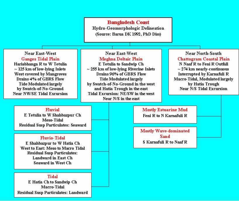
. . . Perhaps – our learning process starts as we begin to develop questions in our mind – like if or when. In computer programming ifs and the answers to such ifs – are used to direct processes in different directions – so does our learning processes. Questions similar like these, reflecting on the past: if I had done things differently . . . if I had been informed differently or were able to see things through my own lens . . . if I had someone powerful on my back . . . so on – and so forth. And intelligent answers to them help us chart future directions. Similarly, such questions can be framed in our mind – at any time – to help examining the pros and cons of making decisions. Sometimes, we fail to ask such questions in time, and mistakes are made – from which recovery becomes difficult. It’s like one of Tagore (1861 – 1941) songs: keno jaminee naa jheta jagelaa naa – saying, why didn’t you wake me up before it was dawn. In one way or another – the consequences of making decisions based on answering ifs –– define the interdependent fluxes in the evolving canvas of life in time, and in the space where one lives – the spacetime. And as we do so, we begin to realize what Benjamin Franklin (1706 – 1790) once said: . . . without continual growth and progress, such words as improvement, achievement, and success have no meaning . . . Starting from these words of wisdom, let us attempt to understand some dynamics of currents in coastal oceans off rivermouths – focusing on the one, off the mouth of Ganges (Ganga) Brahmaputra River System (GBRS; or the GBM system). Needless to say that such understandings – are very imperative to initiate, manage and execute Civil Engineering on Our Seashore – to achieve sound and sustainable goals. Engineering services are involved in one way or another – in the processes of attaining the 17 interconnected UN declared Sustainable Development Goals (SDG). . . . Thought of presenting some findings from the 2nd Chapter of my Ph.D. Dissertation – with a note that unlike in An Alluvial River’s Sedimentary Functions, I am keeping the name Brahmaputra River in line with my Dissertation – although its reach in Bangladesh is known as the Jamuna River. Some aspects of this chapter were presented in the Characterizing Wave Asymmetry, with discussions of some theoretical frameworks posted in Nonlinear Waves. This is the only chapter – which I could not manage time to send the manuscript for journal publication. Other chapters are published: Chap 1 (1991), Chap 3 (1995) and Chap 4 (1994). Facilitated by my major Prof WS Moore, the 2nd Chapter benefited from the works and advice of my Dissertation committee member Prof B Kjerfve. Acknowledging them in gratitude – let me move forward to focus on the main contents of this piece – on coastal ocean currents. In this piece, I am doing this very briefly with some of the interpretations and explanations that accrued from my later experiences and related publications – some of which are summarized and listed in the ABOUT page. Among them, the most relevant publications for this article are: the 1990 IEB Journal Paper on Estuary; the 1991 COPEDEC-PIANC paper; the 1993 Practices and Possibilities; the 1994 Karnafuli River Estuary Hydraulic Behavior; the 1997 Active Delta; the 2001 Suspended Sediment Measurement; the 2002 Geometric Similarity of Deltas; the 2004 Settling Velocity of Natural Sediments; the 2008 Fluid Mud; the 2015 Longshore Transport; and the 2017 Seabed Roughness. It is also enriched by the works done while writing several articles posted in the WIDECANVAS. . . . Before I begin, a short note on The Coastal Force Fields is helpful. The fields represent a playground of many forcings and responses of different time-scales afforded by different constraints – defined by isobaths and the land-water interface at the shoreline/coastline (see more in the Civil Engineering on our Seashore). Together, the system of forces head to reach dynamic equilibrium (see Natural Equilibrium; Water Modeling). According to the force fields defined there – GBRS mouth is governed by forces – that are in dominant actions, but differing in the contexts of both space and time - the Metocean Force Field (MOFF), the Extraterrestrial Force Field (ETFF), the Land Drainage Force Field (LDFF) – are all there, together with the Frontal Wave Force Field (FWFF) – which is active in the proximal shoreline and shallow areas. As well important is the Storm Surge that frequents the coastline often. Currents or velocity fields are generated by the development of pressure gradients generated by the highlighted force fields. They are a manifestation of hydrodynamic interactions – of force and response fields – as depicted in the image of Force Fields in a Coastal System. . . . The Hydro-Geomorphologic Setting – the Processes and Forms. Let me begin by referring to the attached image (it is enriched by some materials discussed in the Coastal River Delta) – that summarizes some of the key hydro-geomorphologic features and processes of Bangladesh coast. The definitions and delineations have been used by many subsequent authors to describe Bangladesh coastline.
The Measurements – the Time, Tide, Site and Season. Let me briefly outline the measurements on which the findings described in this article are based (please refer to Chapter 2 of my 1992 Dissertation for details).
Coastal Water and Wind-driven Circulation. Here is a gist on the nature of changing seawater salinity (see Coastal Water to know aspects of it) at measured stations, and the wind-driven circulation (see Storm Surge to know aspects of it).
Submarine Canyons Refract Tide. The set of measurements in waters between 5 and 20 m isobaths – covering nearly the whole stretch of Bangladesh coastal ocean indicate something very interesting about the refraction of tidal wave by deep submarine canyons.
Tidal Oscillation, Currents and Residuals: The three sets of described measurements are fairly representative of the river hydrograph and the changing monsoonal wind pattern. In spite of a few exceptions, the data indicate some interesting hydrodynamic characteristics of the surveyed area.
There we have it – a brief synopsis of coastal ocean current dynamics off rivermouths – where the actions of tide, seasonal riverine flow and wind conditions (for details see Chapter 2 of my Dissertation) define the force fields. This article is dedicated to celebrate the 51st anniversary of Bijoy Dibash – the Day on 16 December 1971 marks the Liberation of Bangladesh from the tyranny of Pakistani rule. Let freedom loving people from around the world come together to breathe the fresh air of emancipation – by being conscientious, heedful and diligent – whenever – wherever – whatever. And let us do that by remembering Charles Dickens (1812 – 1870), the British writer, novelist and social critic: have a heart that never hardens, and a temper that never tires, and a touch that never hurts. . . . The Koan of this piece: Be mindful what you think, say or do, because the Sun has the habit of not shining on one place for long . . . . . - by Dr. Dilip K. Barua, 16 December 2022 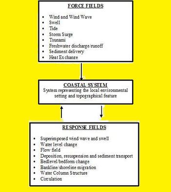 In this piece let us attempt to see in simple terms – the dynamics of coastal systems through a different scientific angle. This angle is the Force Field Theory (or ENERGY FIELD) first proposed by Michael Faraday (1791 – 1867) in 1845 (see The Quantum World; for a short introduction of the concept). A Coastal Engineer’s works, or widely the works of a Civil Engineer belong to the domain of Gravitational Force Field, GFF – formulated by Isaac Newton’s (1642 – 1727) Universal Law of Gravitation (ULG); and its dynamic characterization by Albert Einstein’s (1879 – 1955) General Theory of Relativity (see Einstein’s Unruly Hair). The GFF is a ubiquitous invisible field that affects everything on the Earth’s gravitation field. It defines all the downslope processes, and establishes the necessity of doing work to create upslope events (see Upslope Events and Downslope Processes). We vividly see the gravitational active force in fast flowing streams – and the gravitational restoration force in waves. In all of a Civil Engineer’s works – the universal gravitational acceleration ‘g’ is present (for all practical purposes, g = 9.81 m/s^2 on Earth’s surface). This value appears in almost every relation – with the mass or density (mass per unit volume) of a substance – together they define the weight of the gravitational force. To be in perspective, while GFF defines the Natural World; as a member of the Quantum Field (QF) family, the EMFF is ubiquitous and defines the world of electromagnetism.
Perhaps the dynamics of a coastal system – for that matter of any open system on Earth’s surface – can be viewed for convenience, in terms of external excitation or agitation forces on a system – and its internal balancing responses. Alternatively, this duo represents Action-Reaction Fields – in terms of Newton’s Equation of motion translated into Navier-Stokes Equation (see Seabed Roughness in Coastal Waters). I have presented an early version (shown in the image) of the force-response field concept quite a while ago while giving a seminar at UBC and later at the University of Central Florida – where force and response fields were shown separately defining the dynamics of a coastal system. For simplicity of discussions, I like to discuss the coastal dynamics in terms of five interactive Force Fields: (1) Metocean Force Field, MOFF; (2) Extraterrestrial Force Field, ETFF; (3) Land Drainage Force Field, LDFF; (4) Heat Exchange Force Field, HEFF; and (5) Frontal Wave Force Field, FWFF. The hydro-sediment-seabed dynamics responding to these imposed forces are discussed in these five force fields. I have also included a brief on the Structure Response Field (if structures are present). . . . A different way of looking at the Force Field Systems is through the Hydrodynamic Entropy as proposed in Entropy and Everything Else. All the force fields impart energy into water – transforming its dynamic characteristics. One very obvious example is the effect of a Frontal Wave Force Field – in transforming the dynamic characteristics of the medium – e.g. an oscillatory wave transforming into a translatory wave – generating the cascade of dissipation processes. Let me attempt to refresh our understanding of a coastal system – based on pieces posted earlier: Coastal Water and Civil Engineering on our Seashore. A coastal system where the above interactive force fields function – is defined by two vertical boundaries (or the continuity of such boundaries into one or more depending on the type of physical barriers) and two horizontal boundaries (see more in Water Modeling piece). The horizontals are the water surface through which it interacts with air – and the seabed, where it interacts with bottom resistance or reactive force. The verticals are: the open water boundary through which it interacts with its neighbors – and the shoreline of the topographical resistance or reactive force. One can also define other systems for the convenience of analysis and purpose (see Entropy and Everything Else). . . . Metocean Force Field
Extraterrestrial Force Field
Land Drainage Force Field
Heat Exchange Force Field
Frontal Wave Force Field
. . . Let me finish this piece with a Koan: People are the most important institution. Irrespective of the governing system – if those in power fail to uphold the trust and confidence of this institution – of people’s aspiration and wellbeing – then the governance turns into tyranny. . . . . . - by Dr. Dilip K. Barua, 25 August 2021
There is nothing noble in being superior to your fellow man; true nobility is being superior to your former self. Who can be a better person than Ernest Hemingway (1899 – 1961) – to write this in his skillful way of crafting words in a lucid and attractive style? Sayings similar to this have been penned down in several pieces of WIDECANVAS in different contexts – not to advance is to fall back – change and refinement as a show of intelligence – maturity – adaptation . . . etc. But Hemingway touched upon a very important aspect of human mind. That being taken over by superiority or inferiority complex (see aspects of it, in Some Difficult Things) – inhibits a person’s ability to think and function normally. This piece is nothing about these complexes – but on something that define Nature – in this case, the transmission or propagation of errors or uncertainties in wave loadings on coastal structures. Uncertainty (U), in its simplest term, is just the lack of surety or absolute confidence in something.
Uncertainty Propagation (UP) refers to the transfer of uncertainties from the independent variables into the dependent variable – simply put, from the known to the unknown. It is transferred in an equation or relation – from the individual variables on right hand side – into the dependent variable on the left. More commonly the propagation process is referred to as error propagation. The two – error and uncertainty are often used interchangeably. In quantitative terms, while error refers to the difference between the measured and the true value – uncertainty refers to the deviation of an individual measurement from the arithmetic mean of a set of measurements. As we shall see, the magnitude of propagated uncertainty is a function of the type of equation (e.g. linear, non-linear, exponential, logarithmic, etc). Uncertainty of a parameter implies that, if it is measured repeatedly – one would find that there is no single value – rather a range of random values accrue that deviate from the arithmetic mean (AM, µ) of the measured set. One needs a method or standardization to characterize the scattered deviations. If the deviations are distributed symmetrically about the arithmetic mean – then a Gaussian (German mathematician Carl Freidrich Gauss, 1777 – 1855) bell-shaped curve can be fitted. One property of such a distribution is defined as the Standard Deviation (SD). This is estimated as the square root of variance (defined as the mean of all deviations squared). If SD is normalized by dividing it with AM – the GD turns into Normal Distribution or ND. The normalized SD, σ/µ, termed as the Coefficient of Variation (CV) – is SD relative to AM. Its distribution follows the symmetry about the mean – and as a fraction or percentage, it covers both sides of the mean. It is like the unit of standard deviation – e.g. 1SD unit saying that 68.2% of the data are scattered on both sides of the mean. A high value of CV is the indication of a large scatter about the mean. CVs are due to nature of the variable in their random response to different forcing functions or kinetic energy (see Turbulence) – and are therefore termed as random uncertainty or simply uncertainty (see more on Uncertainty and Risk). It is the signature characteristic of the variable – and is due to many other factors including the applied measuring or sampling methods. Not all variables follow the Gaussian distribution (GD), however. For example, a discrete random variable, like an episodic earthquake or tsunami event – are sparse and do not follow the rules of continuity, and is best described by Poisson Distribution (PD, in honor of French Mathematician Simeon Denis Poisson, 1781 – 1840). An ideal example of a continuous variable that follows ND is coastal water level. In this piece, all applied variables are assumed to follow ND. Here are some typical CVs from R Soulsby (1997): water density, ±0.2%; kinematic water viscosity, ±10%; sediment density, ±2%; sediment grain diameter, ±20%; water depth, ±5%; current speed, ±10%; current direction, ±10o; significant wave height, ±10%; wave period, ±10%; and wave direction, ±15o. Error or uncertainty propagation technique has been in use for long time dating back to the now known method since 1974 (G Dalquist and A Bjorck). The most recent treatment of the subject can be found in BN Taylor and CE Kuyatt (1994) and in AIAA 1998 (The American Institute of Aeronautics and Astronautics). The propagated uncertainty has nothing to do with the scientific merit of a relation or equation; it is rather due to the characteristic or signature uncertainties of the independent variables – which according to the UP principle must propagate or transmit onto the dependent variable. . . . This piece is primarily based on four pieces posted earlier: Uncertainty and Risk; Wave Forces on Slender Structures; Breakwater; and The World of Numbers and Chances; and three of my papers:
Before moving on, let me try to demonstrate how UP principle works – by discussing a simple example. Suppose, we consider an equation, X = Y^2 * Z. Let us say, the variables Y and Z on the right hand side of the equation have known CVs: ± y, and ± z, respectively. How to estimate the CV of X? According to the UP principle, the CV of X can be determined as the square root of x^2 = 2^2*y^2 + z^2. As an example, suppose, y = ±10%, and z = ±5%; then x must be equal to 20.62%. Further, a pertinent question must be answered. Why Uncertainty? or Why Uncertainty Propagation? The relevance of the questions stems from the quests to develop confidence of the relations or equations one uses to compute and estimate parameters for everything – from the science of Nature to Social Interactions to Engineering and Technology. These relations developed by investigators after painstaking pursuits convey theories and principles mostly on deterministic paradigm. But, things in Nature are hardly deterministic – which means the independent variables on which a relation is based – suffer from uncertainties of some kind due to their stochastic characteristics and variability. These uncertainties associated with the independent variables must be accounted for in the dependent variable or computed unknown parameter. Uncertainty propagation method developed over a period of many years – gives answer to the questions (see more on Uncertainty and Risk, and The World of Numbers and Chances). In engineering design processes, the traditional method of accounting for uncertainty is done simply by including some redundancy in the system – by the so-called factors of safety – conspicuously described and/or inconspicuously embedded in some practices (for example, using maximum load and minimum strength; and summation of different loads together although they may not occur simultaneously). Further elaboration on coastal design processes can be found in Oumeraci et al (1999), Burcharth (2003) and Pilarczyk (2003). They scaled the processes of design as: Level 0 – deterministic approach; Level I – quasi-probabilistic approach; Level II – approximate probabilistic approach; and Level III – fully probabilistic approach. In the Level 0 approach, parameter uncertainties are not accounted for, instead experience and professional judgment are relied upon to implant redundancy. This practice as a way of developing confidence or assurance – represents in reality – a process of introducing another layer of uncertainty – partly because of heuristics associated with judgments. Or in another interpretation, it amounts to over-designing structure elements at the expense of high cost. For the other three Levels, a load-strength reliability function is defined in different scales to account for parameter uncertainties. A note on significant wave height uncertainty is warranted. Although a typical ±10% is recommended by Soulsby, in reality the uncertainty can be varied. The reasons can be traced to how the local design significant wave height is estimated. Some likely methods that affect uncertainty are: (1) the duration, resolution and proximity of measurements to the structure; (2) extremal analysis of measurements to derive design waves; (3) in absence of measurements, applied analytical hindcasting or numerical methods to estimate wave parameters; and (4) applied wave transformation routines or modeling. Due to these diverse factors affecting uncertainty, instead of considering one uncertainty, this piece covers a range from10 to 30%. . . . Uncertainty of Wave Loading on Vertical Pile This portion of the piece starts with 2008 ISOPE paper and Wave Forces on Slender Structures. Unbroken waves passing across the location of a slender structure (when L/D < 1/5; L is local wave length and D is structure dimension perpendicular to the direction of force) cause two different types of horizontal forces on it. The basis of determining them is the Morison equation (Morison and others 1950). Known as the drag force in the direction of velocity, the first is due to the difference in local horizontal velocity head or dynamic pressure between the stoss and the wake sides of structure. The second, the inertial force is caused by the resistance of structure to the local horizontal water particle acceleration. Both of the Morison Forces have their roots in Bernoulli Theorem (Daniel Bernoulli; 1700 – 1782) – and as one can imagine, they are a function of water density – and of course, the structure size. The horizontal Drag Force: a function of water density, structure dimension perpendicular to the flow, water particle orbital velocity squared, and a drag coefficient. The horizontal Inertial Force: a function of water density, structure cross-sectional area, water particle orbital acceleration, and an inertial coefficient. To demonstrate UP of wave loadings at the water surface on a cylindrical vertical pile of 1 meter diameter – this piece relies on the same example wave discussed in Linear Waves; Nonlinear Waves; Spectral Waves; Waves – Height, Period and Length and Characterizing Wave Asymmetry. This wave, H= 1.0 m; T = 10 second; d = 10 m; has a local wave length, L = 70.9 m and Ursell Number (Fritz Joseph Ursell; 1923 – 2012) = 5.1; indicating that the wave can be treated as a linear wave at this depth. Other used and estimated parameters are: water density = 1025 kg/m^3; amplitude of horizontal orbital velocity at surface = 0.56 m/s; and amplitude of horizontal orbital acceleration at surface = 0.44 m/s^2. In addition, while using most typical uncertainties proposed by Soulsby – the Us of wave length, orbital velocity and acceleration have no typical values – therefore they are derived in the 2011 paper and in this piece applying the basic UP principle. The results of uncertainties in wave loadings are shown in the two presented images – one for the drag force (UDF), the other for inertial force (UIF). They are shown as a function of uncertainties in measured wave heights (U_H) for U_water density = 0.2% and U_linear dimension = 5%, with estimated U_cylindrical pile area = 10%. Since the uncertainties of coefficients (U_Cd and U_Cm) are not known, the images show three cases of them, 10%, 20% and 30%. Here are some numbers for U_H = 10% and 30%.
. . . Uncertainty of Wave Loading on Breakwater Armor Stone This portion of the piece primarily depends on materials developed and presented in the Breakwater (BW) piece posted earlier, as wells as on my 2011 paper. The state-of-the-art techniques in determining armor stone masses or sizes of rubble-mound breakwater and shore protection measures – rely either on Hudson Equation (RY Hudson 1958) or on VDM Formula (JW Van der Meer 1988). The applicability and relative merits of the two methods are elaborated in the Breakwater piece. For simplicity of analysis, I will focus on the uncertainty of Hudson Equation. This equation relates Stability Number to the product of a stability coefficient (KD) and a BW side slope factor. The equation provides estimates of median armor stone mass as: a product of the stone density and wave height cubed – divided by the product of KD, side slope factor, and relative stone density cubed. It is assumed that armor stone is forced by H = 1.0 m on the BW seaside slope = 1V:2H; with stone density = 2650 kg/m^3 and water density = 1025 kg/m^3 giving a relative stone density = 2.59. The uncertainties of relative density and side slope factor are not known, they are estimated at 2.01% and 7.1% using basic UP principle. The crux of the problem appears on defining the KD values. The recommended KDs vary from 1.6 for breaking to 4.0 for non-breaking wave forcing (USACE, 1984). Melby and Mlaker (1997) reported that the KD values have uncertainty of some ±25%. In this piece the uncertainties median armor stone mass U_M50 for KD uncertainties ranging from ±10% to ±25% are investigated. Some estimated numbers are:
. . . The Koan of this piece on this International Jazz Day: What seems to be perfect to an ordinary eye – is never finished, never perfect in the creator’s eye. The creative works continuously explore, experiment and search for something – that never comes to the satisfaction of the creator. . . . . . - by Dr. Dilip K. Barua, 30 April 2021 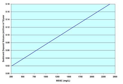 A harbor is a water basin of tranquil or tolerable wave and current climate, and of sufficient water depth in which a maritime or inland vessel (let us use this general term, but when Dead Weight Tonnage or DWT ≥ 500, a vessel is known as a ship) can operate safely. Maritime harbors are selected from the deep shoreline areas sheltered naturally, or are created artificially (see Flood Barrier Systems). The artificial harbors are configured and engineered within an ambient water body at the shoreline by dredging and installing suitable structures (see Breakwater). The purpose in each case is to locate a maritime port or marina within it (see Ship Motion and Mooring Restraints; and Propwash). For the convenience of design and operation, a harbor is classified and distinguished as deep-draft (water depth > 15 ft or 4.6 m), and shallow-draft or small-craft (water depth < 15 ft or 4.6 m). Many artificial harbors have one inlet to allow influx and efflux of water and sediment into the basin (a semi-enclosed basin that allows restricted/controlled entry and exit of matter and energy, see Upslope Events and Downslope Processes); and entry and exit of vessels. The layout of the structure – and the location, width and depth of the approach channel as well as of the harbor itself are designed by addressing such constraints as – ambient wave, current and sediment climates, and the largest allowable vessel designed to call at the port.
. . . In this piece, let us attempt to discuss and understand the sedimentation rates of harbors in simple terms. Sediment transport dynamics and sedimentation pose a complicated problem. But ballpark estimates and numbers are always handy and useful to conceive and study the feasibility of a project. To that end, some methods and pieces of data are selected and blended in this piece. The purpose is to demonstrate the usefulness of some simple analytical models that can be used as a handy tool to picture a high-level impression of possible harbor sedimentation. The magnitude of sedimentation problem can be appreciated if one considers worldwide dredging operations. Maintaining enough water depth within the harbor and keeping the approach channels navigable – are some of the requirements that let flourishing of huge dredging industries. These two major demands, together with the erosion prevention and value-adding beach nourishment works, and others – have yielded the global dredging industry to an annual turnover of some $5.6 billion. I will try to come back to discussing different interesting aspects of dredging at a later time. Among others, this piece is primarily based on: RB Krone 1962; Delft Hydraulics publications (E Allersma 1982; WD Eysink and H Vermass 1983 and WD Eysink 1989); R Soulsby 1997; USACE 2002 EM 1110-2-1100 (Part III) and 2006 EM 1110-2-1110 (Part II); I Smith 2006; and my own works on fine sediments and sedimentation (Fluid Mud 2008; and Settling Velocity of Natural Sediments 2004) published in the Journal of Hydraulic Engineering, and Journal of Waterway, Port, Coastal and Ocean Engineering, respectively; Seabed Roughness; and two papers presented at the International Symposiums on Coastal Ocean Space Utilization: COSU 1995 and COSU 1993, and my paper at the 24th International Conference on Coastal Engineering, Kobe, Japan, ICCE 1994. The Hydraulics of Sediment Transport and Resistance to Flow posted earlier laid out some fundamentals of sediment behavior and transport. . . . Configuring the layout of a harbor entrance needs careful optimization exercises and analyses – on the one hand, it has to provide effective diffractive energy dissipation of incoming waves – on the other, it has to minimize the formation and strength of current eddies at the entrance, and sedimentation inside the basin. Filling and emptying tidal currents at a harbor entrance are usually an order of magnitude less than the ambient tidal current. Their magnitudes depend on the size of the basin and entrance. Eddies – more vigorous during changing current directions – are undesirable for at least two primary reasons. The first is to minimize navigation hazards – to vessels entering and leaving the port. The second is to minimize scour and formation of sandy bars. Exercises to engineer a detailed and optimal layout include physical scale modeling and/or numerical modeling. Such exercises, especially the efforts of numerical modeling (see Water Modeling) are becoming increasingly common not only for optimizing harbor entrance layout, but also for visualizing the sediment morphodynamics, sedimentation and other aspects of harbor hydraulics (e.g. Ports 2013 paper). Before moving on, let us have some words on tidal action. It is assumed that actions attributed to short-waves (see Ocean Waves and Linear Waves) and vessel generated wake-waves are minimal – a valid assumption for all harbors. The main concern of harbor sedimentation processes is the behavior of Suspended Sediment Concentration (SSC) that has a positive gradient from low at top to high at bottom of the water column. As flood and ebb currents reach threshold for erosion and resuspension during a tidal period – sediments are picked up from the seabed and are transported (coarser fraction close to the bed; fines up in the water column) back and forth by the current. Similar but opposite episodes happen, as flood and ebb currents slow down to reach deposition threshold. Suspended sediments have the opportunity to settle down during such slack water periods (SWP) – with more chances for sediments close to the bed than those up in the water column. However, there is often a settlement lag or incoherence between the slack water and actual deposition (see more in my 1990 Elsevier paper). . . . Let us now dive down into the core issue of this piece. A harbor faces at least two types of major sedimentation problems. The first is the formation of localized shoals or sandbars at and around the entrance due to the scouring actions of eddies, and the sudden drop in flow velocities. These shoals mostly of sandy materials are often attached to the shoreline as a side bar or develop as middle bar(s). They mostly develop when the harbor entrance is located on littoral shores (see Managing Coastal Inlets) – and are usually termed as flood-tidal and ebb-tidal deltas (see Coastal River Delta and Managing Coastal Inlets). The dynamics of such sandy shoals, bars or deltas can best be discerned from the piece on The Hydraulics of Sediment Transport. The focus of this piece is on the second type of sedimentation problem. It is the sedimentation of fine sediments within the harbor basin. This sedimentation (a phenomenon of suspended sediments having very low settling velocities) is somewhat uniform due to the relatively weak circulation within the harbor basin – but is often less in areas of relatively high currents than in remote areas of stagnant water. It is highly problematic when a harbor is located within Turbidity Maximum (TM) zone (1990 Elsevier paper). The presence of TM in the tide-dominated east shore channels and waterways of the Ganges-Brahmaputra-Meghna (GBM) River mouth has shown very high siltation rates of fine sediments (1997 Taylor & Francis paper). Observations at the mouth of Karnafuli River estuary showed a positive correlation between the Surface Suspended Sediment Concentration (SSSC) and tidal range (TR) – indicating that the resuspension actions of tidal currents are directly related to tidal range. This correlation ends up yielding an exponential relation between SSSC and TR (ICCE 1994). The fitted relation shows, for example, that at mean neap-tidal TR = 1.7 m, SSSC = 154 mg/L; and at mean spring tidal TR = 3.8 m, SSSC = 1912 mg/L. The gradual but slow filling up of the basin is highly dependent on the concentration of sediment suspended (in textures of fine sand, silt and clay) of influx water. For the convenience of discussion, let us spilt the piece in two: (1) the first is on sedimentation of granular (silt-sized particles) materials; and (2) the second is on sedimentation of silty/clayey materials that are affected by aggregation and flocculation. The provided estimates represent only a high-level first-order magnitude – afforded by some approximations and assumptions. And to be simple yet realistic of a deep-draft harbor, let us use most of the same inlet/basin/tide parameters (inlet depth 15 m; harbor depth 10 m; semi-diurnal tidal period 12.42 hours; and tidal amplitude 1 m) as described in Managing Coastal Inlets – for a large harbor area of 1 million square meter; and an inlet length and width of 100 m and 300 m, respectively. A tide of this amplitude at 15 m water depth, causes a passing peak depth-averaged current of about 0.81 m/s in front of the harbor. A rough estimate shows that for a harbor of this size at this tidal condition – the turnover time (the time required to tidal flushing out 63% of the harbor water volume) is about 3.2 days. . . . Sedimentation of Suspended Particulates
Sedimentation of Aggregated Particulates This part of the piece is based mostly on my published papers: the 1994 ICCE 24th; and the COSU 1993 and 1995 papers. The published works are based on some site-specific information; and are therefore primarily applicable for situations and conditions in which they were derived. But the approach and methodology can be applied elsewhere with some assumptions for cases – of tide-dominated estuaries, bays and waterways dominated by fine seabed sediments. Let us attempt to see some applications of the gained experience in simple terms. They are supplemented by my discussions in 2004 and 2008 publications.
. . . Before finishing I like to tell a story the Buddha (624 – 544 BCE) told to a congregation of monks and lay people. He did this in context of the 4th Buddhist precept of Right Speech (see Revisiting the Jataka Morals – 2). Once an angry and hateful person used very harsh and abusive words to the Buddha. Instead of getting provoked, the Buddha calmly listened and told the man to take back his abusive outburst. The man was dumbfounded hearing such an unusual reaction. The Buddha then said: Hold it there. If a person gives a gift to another, and if the second person refuses to accept the gift, to whom the gift belongs? The man replied: it belongs to the first person. The Buddha said: so, my friend you must take back the abusive language you have used, because it belongs to you and I refuse to accept it. Then the Buddha delivered some words of wisdom to the congregation: if someone spits against the sky, the spittle returns back to the spitter. So, be mindful. If you use an abusive or unwholesome speech, it gets back at you. . . . . . - by Dr. Dilip K. Barua, 23 November 2020 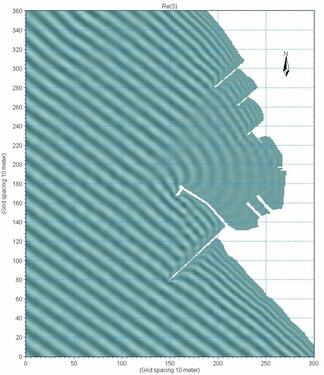 Ever since the 1978 failure of a massive breakwater (BW) in Port Sines, Portugal – coastal engineers around the world went back to reviewing the BW design approaches and methods. During my studies at Delft in 1982 – the event and the possible lapses and causes of its failure – came for discussions again and again in coastal engineering lectures. The Sines Deepwater (~ 50 m) BW was designed and constructed of massive 42 tonne armor-layer dolos (dolos are pre-fab concrete units, designed to achieve good interlocks and stability when placed randomly – each unit has three stems, the central and the two twisted ones on ends) to withstand waves up to 100-year extreme of 11 m high significant wave (see Spectral Waves for definition). But near the end of the construction period – a storm that registered a lower wave height, dislodged about 2/3rds of the units – and some subsequent less powerful storms did the rest of the work by destroying the BW.
The risk of failure, the scale and cost of such massive structures – have generated renewed research interests in coastal labs around the world. Physical scale modeling tests – such as those in the massive Delta Flume in Emmeloord (the Netherlands), and in the CERC (Coastal Engineering Research Center) facilities in Vicksburg, Mississippi were some of the examples. The efforts resulted in the refinement of existing formulae and coefficients, and yielded new ones. . . . In this piece let us attempt to understand some interesting aspects of BW engineering. Engineering literature is full of materials on various aspects of BW planning, loading, stability, designs, and effects assessments. Among them, the following lists have most of the resources one needs for breakwater engineering: (1) Random Seas and Design of Maritime Structures (Y Goda 2000); the USACE (United States Army Corps of Engineers) (2) 1984 Shore Protection Manual (SPM); and its reincarnation, Coastal Engineering Manuals (CEM): (3) the 2002 CEM (EM 1110-2-1100 Part II; Chap 8 – Hydrodynamic Analysis and Design Conditions), (4) the 2006 CEM (EM 1110-2-1100 Part VI; Chap 5 – Fundamentals of Design, and Chap 6 – Reliability Based Design of Coastal Structures); (5) the 2007 Rock Manual (C683, the use of rock in hydraulic engineering, 2nd ed.) of EUROCODE, CIRIA (Construction Industry Research and Information Association) and CUR (Civil Engineering Research and Codes, the Netherlands); the JW Van der Meer publications, starting with his (6) 1988 Ph.D. Diss. (Rock slopes and gravel beaches under wave attack, Delft Univ. of Technology, the Netherlands, Delft Publication No. 396); and his (7) 1992 Delft Lecture Note, Conceptual Design of Rubble Mound Breakwaters; (8) RY Hudson 1958 (Design of quarry-stone cover layers of rubble-mound breakwaters, hydraulic laboratory investigation, Research Report 2-2, Waterways Experiment Station, Vicksburg, MS); and (9) R Iribarren 1938 (Una Formula Para el Calculo de los Digues de Escollera, Technical Report HE 116-295, University of California, Berkeley, CA). On 2D Wave Diffraction Modeling suite: (10) the 2005 Bouss-2D Wave Model in SMS, ERDC/CHL CHETN-I-69/70; (11) the 2007 Delft3D-Wave, TU Delft and Delft Hydraulics; and (12) the 2008 Waves Modules, DHI (Danish Hydraulic Institute). Different aspects of BW engineering are highly elaborate – I will briefly focus on some selected portions of them in simple terms. An overview of civil engineering works on our seashore (see Civil Engineering on our Seashore), and of barrier systems engineering (see Flood Barrier Systems) were posted earlier – that laid out some basics of coastal engineering (CE) works. . . . A BW generally refers to an in-water self-standing coastal protection or defense structure – shore-attached, detached or offshore. It belongs to the Water Barrier group of structures (see Flood Barrier Systems) in coastal engineering; and may define a system when multiple BWs and functions are integrated together as a package. The purpose of a BW is to diffract, break and obstruct the continuity of an incoming wave – in order to create a tranquil or shadow zone of minimal or no wave activities behind it. Although the term is primarily applied to describe coastal protection or defense structures against wave attack, the underlying concept is similar – for example, in breaking the flow of a river current to protect an inland harbor or river bank erosion from current forcing (collectively known as river training structures). The functional properties of a BW are achieved by designing a suitable layout and dimension – the size of which falls into the definition of a large structure – with its dimension, D scaling with the local wave length, L such that D/L > 1/5 (see Wave Forces on Slender Structures). This means that a BW has a significant presence in the surrounding hydrodynamic field – in diffraction, deflection, reflection, transmission, absorption and scattering of waves, currents and alluvial sediment transports and dispersion. One important aspect of BW configuration – in terms of hydrodynamic loading – is the convergence and divergence of wave energies. The convergence – in particular, at the convex bends and at BW heads – implies that those places must be stronger than the rest of the structure to withstand amplified wave loading. . . . Breakwater Types and Functions The necessity for a minimal wave zone can be varied – in port applications, the purpose is to create a harbor where vessels and ships (see Ship Motion and Mooring Restraints) can safely navigate in and out – and moor to load and unload cargoes and people. The second most important necessity is to protect a shore from wave erosion and beach degradation, or to prevent entry of unwanted sediments into a harbor. BWs are classified as two basic types: Floating and Fixed. Floating BWs are pontoons tethered in position either by guide piles, or by chains anchored to the seafloor. A pontoon acts as a deterrent of, or as a low-pass filter to the incident waves (mostly short-periods ~ 4 s) – with the additional use as a loading/unloading platform. They are mostly applied in low wave-climate areas to design marinas where small pleasure boats can be safely secured on several inside finger floats. Different aspects of this type of BW – incident wave attenuation efficiency and transmission are discussed in the Wave Structure Interactions & Scour piece. The primary focus of this piece is Fixed BW. Breakwaters anchored to and founded on the seabed – as statically or dynamically stable hydraulic structure define a fixed BW. Depending on the scale of project and purpose, as well as on the prevailing hydrodynamic and wave climate, a fixed BW structure can be built by sheet pile walls, caissons (a concrete box or boxes filled with sand), rubble mounds, or combinations of them. Typically, caisson breakwaters can be a vertical face type, a composite type when the caisson sits on top of a raised platform built by rocks/rubbles, a perforated vertical face type (perforations eliminate wave reflection from the vertical wall), and armored caisson type (the seaside of the caisson is protected by rock armor units). Both sheet pile and caisson structures need quarry rock scour protection at seabed. . . . Fixed BW can be classified according to the magnitude of a Stability Number – defined as a ratio of wave height (H) to the product of armor unit relative density (Δ) and a characteristic dimension (D) of the unit or N_s = H/ΔD. When N_s ≤ 1, it falls into the category of a statically stable monolithic massive defense structure such as caissons and seawalls (in this case D is the height or width of the structure). All other structures including the rubble mounds and the shoreline itself are mostly dynamically stable with N_s > 1 (for rubble mounds, D = D_n50, the 50th percentile nominal rock diameter). In a dynamically stable structure, hydrodynamic forcing is assumed to cause profile changes in various degrees – with the displacements of rocks from a relatively unstable position to new stability. While this process goes on, the integrity of the structure remain largely unaffected or intact. However such structures succumb to failure – when large amounts of armor rocks are broken or are carried away exposing the underlayers and foundational core. BWs can be designated into four vertical zones according to their exposure to the hydrodynamic loading. They are: the Zone I – the bottom foundational zone below the level of Mean Low Water (MLW); the Zone II – the tidal zone from MLW to the Mean High Water (MHW), loading on this zone is very frequent and determines the longterm structural stability; the Zone III – the higher high water zone from MHW to the design level, wave attack on this zone is less frequent but of high impact; and the top Zone IV subjected to the effects of runup and overtopping. Shore perpendicular breakwaters attached to the shore are mostly conceived to serve beach management purposes. They are termed as Groins or Groin Systems, and have a range of typical shapes (Straight, T, Y, L, etc.) – the selection of which depend on the purpose and effectiveness. These types of breakwaters interrupt littoral transport, and attenuate the effects of onshore waves. They are usually low crested and are constructed of low-cost quarry rocks and runs. Literature and manuals suggest different planning approaches of such structures. For Groin Systems, the length of each unit is usually transitioned from short at the updrift side to the full length at the downdrift side. The spacing between each Groin usually scales with the length: the spacing is some 2 to 3 times the Groin length. Shore parallel detached breakwaters – as a way to manage beach erosion and littoral transport – are often identified according to its location with respect to the shoreline. A parameter (L) defining a ratio of breakwater distance from the shoreline (X_off), and the 80% of surf zone width (S_80, note that about 80% of littoral transport occurs within the surf zone; see The Surf Zone processes), or L = X_off/S_80. When L ≤ 0.5, the breakwater is classified as a Beach BW (it protects the foreshore without significantly altering the littoral transport). A Coastal BW is defined when 0.5 < L ≤ 2.0 (intervenes the littoral transport to prevent beach erosion). At L > 2.0, it is known as Offshore BW. This type must be highly robust to withstand high waves and to interrupt and diffract incoming waves. A fixed BW can also be classified according to the elevation of its crest from the still water level. In broad terms, two types can be identified: the emergent and the low crested breakwaters (LCB). The crest height of an emergent BW is usually high to prevent overtopping or to allow limited spray (breaking waves spray out into air) overtopping – and must take account of design storm surge height, wave set-up, wave run-up, height to compensate BW settlement and a freeboard on top of the design water level. If installed, the concrete cap of an emergent BW (usually used for utilitarian purposes) must be protected against overtopping damages by providing a crown wall. LCBs have various forms and heights depending on the desired limitations of overtopping – and the requirement to achieve certain wave attenuation goals. There are those that allow green overtopping (submerged BW acts as a weir transmitting a portion of the wave energy), and those that emerge and marginally submerge depending on the water level – thus allowing different categories of overtopping. . . . Wave Diffraction by Configuring the BW Layout Diffraction is a process of bending the wave energy by obstructing its direct or head-on propagation. Waves lose a portion or all of its energy while bending from the illuminating zone to the shadows. Engineers use this property of wave behavior to design an area of low-energy wave environment so that vessels and ships can moor safely to load/unload cargoes and people – or to protect a shoreline from high energy wave actions and erosions. The ratio of diffracted (Hd) and incident (Hi) wave heights defines the diffraction coefficient, Cd = Hd/Hi. Characterization of the incident hydrodynamic field in quantitative terms must begin with a clear qualitative understanding of the wave and sediment climate systems of the area. The a-group and b-group of activities shown in the coastal engineering envelope (see Civil Engineering on our Seashore) are the ones to start with. They include: use of longterm timeseries measurements from moored buoy or other platforms (in absence of such measurements, Wave Hindcasting techniques are used, if necessary based on Beaufort Wind Scale) together with analytical and physical and/or numerical modeling. Before the times of digital computation and numerical modeling, engineers used diffraction diagrams and analytical models to determine diffracted wave heights. The Weigel (RL Weigel 1962) diffraction diagrams included in the SPMs and CEMs, and simple analytical models (Goda and others) are some examples. A simple illustration using the Goda relation, would show that an illuminating (a) 3-m, 8-sec head-on wave at 10-m water depth, would diffract to 0.34 m (Cd = 0.112) in the shadow zone at –60 deg (the direction refers to the direction of wave orthogonal approach). Modeling activities search for an optimal layout that would diffract the incoming waves to a tolerable height or energy level behind the BW. Physical scale modeling is somewhat a thing of the past as it involves considerable efforts and cost (however massive projects often require it). In contrast, modern practices of optimizing the configuration of a BW layout mostly rely on numerical modeling. First, the regional wave climate is established by wave action modeling – that lays out the boundary conditions for the detailed modeling including the outlines for most probable forcing scenarios. The most effective way of detailed layout optimization is by Mild Slope or Boussinesq (French mathematician and physicist Joseph Valentin Boussinesq; 1842 – 1929) wave modeling – an example of such an application is shown in the attached image. I love the beauty of Boussinesq modeling approach – its phase-resolving capability to analyze the non-linear wave fields close to the shore, etc. I had the opportunity to use it in multiple occasions – the results of one such application are published in my Ports 2013 Conference paper. While the capabilities are real – there are also many limitations and constraints of what a numerical model can or cannot do – therefore one should be careful in interpretations of model results, and their uncertainties. Some aspects of these issues are outlined in the Water Modeling piece. For the sake of brevity, the rest of this piece will primarily focus on rubble mound BW and designing armor rock size. . . . Rubble Mound Breakwaters Rubble mound breakwaters represent a triangular (trapezoidal to be exact with thick peak) prism with its base at the seabed and its triangular peak rising to a certain height above or below the still water level (SWL). The thickness of the peak is structurally required to have the dimension of 3 armor rock sizes, often equipped with a concrete cap and a seaside crown wall for an emergent BW. The advantage of a rubble mound is its capacity to absorb and dissipate the wave breaking energy – the dissipation is ensured by the porosity of armor layer. It is a relatively cost-effective simple structure with the sides laid out in symmetric or asymmetric slope configuration. The slopes must be flatter than the rock angle of repose or internal friction (~ 1V:1.25H). In the case of an asymmetric triangle, the seaward side slope is usually flatter than the harbor side. Let us attempt to see some aspects of this structure in simple terms. Stability of an Armor Unit. The crucial step in BW engineering is to address the stability of armor rocks or concrete units placed (randomly by dumping, or one-by-one in regular orders) on the rubble mound slope. The hydrodynamic loading of a breaking wave must be balanced by the armor unit weight resting on a slope and held in place by neighboring units and the foundational core. The loading is primarily caused by breaking wave drag and lift forces (inertial forces are negligible, see Wave Forces on Slender Structures). These forces translate to the wave height when breaking water particle velocities become a square root function of H (see Tsunami and Tsunami Forces). In essence, the dynamic stability of armor units depends on a multitude of factors – related to (a) Wave Forcing, (b) Rock Properties and (c) Structural Integrity. They are:
. . . Hudson Formula (RY Hudson 1958). The next breakthrough came from flume tests in the CERC lab facilities at Vicksburg, Mississippi. The derived relation, promoted by SPM manuals and has been in use for long time was the Hudson formula. It simply related N_s to the product of a stability coefficient and slope factor. The formula is based on flume tests relying on the actions of broken waves on non-overtopped permeable core BW slope. SPM manuals prescribed different applicabilities of this formula and provided different tabulated values of the stability coefficient. Although the formula was derived using regular waves, the manual prescribed to use significant wave height (Hs) in the 1977 manual – and changed it to the 10th percentile significant wave height (1.27Hs) in the 1984 manual and in subsequent CEM editions. The limitations of this simple formula are often cited as: (1) probable scale-effects from small model tests; (2) use of regular wave loading only during testing; (3) the effects of wave period and storm duration not accounted for; (4) damage level is not well-defined; and (5) primarily meant for non-overtopped permeable core structure. However, to ensure wide applicability, all these limitations (as we shall see except the wave-period effect) are accounted for, and lumped into the stability coefficient. The example (a) broken wave, when acts on a 1V:2H BW slope, the 1977 formula yield a rough quarry rock armor unit mass of 4.5 tonne with no damage. It nearly doubles to 9.2 tonne when the 1984 formula is used. . . . Van der Meer Formula (JW Van der Meer 1988). Van der Meer (VDM) for his PhD thesis conducted elaborate lab tests in the Delta Flume. His derived formula is more complex than Hudson’s. And N_s is related to additional factors – by taking into account of the effect of wave period, wave breaking type, permeability, damage level, and storm duration. VDM formula is tested for wave steepness from 0.005 to 0.06, and with the maximum wave numbers of 7500, at which the forces on the armor unit reach equilibrium (meaning that no more damages could occur with further increase in the number of waves). Let us see how the VDM formula predicts rough quarry rock armor size for the example wave. The (a) wave breaks on the 1V:2H BW slope as a plunging breaker (see The Surf Zone). For 4000 waves on an impermeable core with no damage, the required VDM unit mass is 6.7 tonne (note that this size is smaller than what is required by the 1984 Hudson). If the wave period is increased to (b) 12-sec, the wave breaking type is still plunging, but then the mass increases to 12.7 tonne. For this particular wave forcing, it turns out that the Hudson 1984 formula is conservative for wave periods ≤ 9.7 sec. For heavy storms characterized by long period waves, the VDM formula is appropriate. . . . Materials. As an alternative to quarry rock, engineers resorted to lab testing to develop different interlocking shapes of concrete units. In most cases, investigations leading to finding such units became necessary when suitable sizes of quarry rocks (most commonly used densities: rock 2.65 tonne/m^3; water 1.025 tonne/m^3; 1 tonne = 1000 kg) could not be identified and found for high wave climate areas – in cost-effectiveness, quantities, qualities and energy dissipation. Concrete units allow engineers to design steep slope (~ 1V:1.5H) rubble mounds, thus affording significant cost savings in relatively deep waters. The units are usually reinforced when the required mass of each unit is heavier than about 10 to 20 tonne (often constrained by the placing equipments and methods). Many countries have developed their own tested shapes, some common examples include (with the year and the countries of development): Tetrapod (France 1950), Tribar (USA 1958), Stabit (UK 1961), Tripod (the Netherlands 1962), Dolos (Republic of South Africa 1963), Seabee (Australia 1978), Accropode (France 1980), Shed (UK 1982), Core-loc (USA 1996), and Xbloc (the Netherlands 2003). . . . I like to stop at this by noting many other aspects of rubble mound BW engineering that accompany design specs. In brief they include:
There we have it. Perhaps some moments of thoughtful reflection and reckoning from all of us are useful – on something as miniscule as a microbe virus yet powerful enough to shatter the confidence in our protective capability of public health. And on something – that opened a terrible flaw in otherwise assumed as civilized systems and norms – but which in reality were nothing but artificial covers on the hidden wounds inflicted by many years of skewed socioeconomic policies promoting asymmetry and inequity. On top of that climate warming is heading towards unsustainable instabilities and trends; and information abuses and malicious internet viruses are at an alarming stage of threatening public security and privacy. With all these, it is no surprise to hear global calls – loud and clear, for the strengths of wisdom, mutual respect and unity. . . . With that, let me finish this piece with a Koan: Nothing compares with the fury of jealousy, arrogance, anger and hatred – when built within the systems of power or is tolerated – it unleashes the ruthless monster of cruelty and brutality that burns everything it comes close to. . . . . . - by Dr. Dilip K. Barua, 19 June 2020 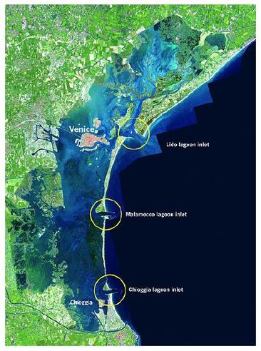 In an earlier piece, Civil Engineering on our Seashore, I have presented and broadly outlined the Coastal Engineering Envelope where several civil engineering measures were shown – that cater to the needs for protecting and developing the seashore. A brief of some 24 different kinds of coastal and port hydraulic structures were listed there. On this piece let us attempt to learn about the Storm Surge Barrier – but in a wider context of Flood Barrier Systems. The barriers as a way of managing water and floods – have two basic engineering components. The first is the dike on low lands, connected to the second component – the gated stream/river/estuary/waterway closure structures. The works represent a system that accounts for many engineering challenges – hydraulic, structural, geotechnical, and risk assessment – as well as impacts on the ambient environment defined by local Fluid, Solid and Life systems (see e.g. Environmental Controls and Functions of a River). In the back drop of Warming Climate with consequent Sea Level Rise, flood barrier systems are becoming increasingly relevant – as one of the management Strategies to cope with the threatening rising sea, and increasingly frequent and intense storm surge.
This piece is built upon materials gleaned from several sources and websites. Unless specified otherwise, they include the following. On river floods: Hydraulic Design of Flood Control Channels, USACE EM 1110-2-1601; Hydrologic Frequency Analysis, USACE EM 1110-2-1415; and Design and Construction of Levees, USACE EM 1110-2-1913. On coastal flood/storm surge: Storm Surge Analysis and Design Water Level Determinations, USACE EM 1110-2-1412; Hurricane and Storm Damage Risk Reduction System Design Guidelines, USACE; and TUDelft (VSSD) Breakwater and Closure Dams (2008, 2nd ed). . . . Before jumping on to discussing the flood barrier systems – perhaps it would be instructive to begin by introducing the Water Barrier concept in a broader context. Because all barriers under this generic term, and in the capacities of a hydraulic structure – have one common purpose – that is to protect an area from the onslaught of water actions. These protections can simply be sorted out against the actions of:
Some common preventative soft and hard engineering measures usually installed for protections against such actions are listed in the Civil Engineering on our Seashore. Perhaps it is helpful to group them pertaining to specific water actions – together with an outline of common assessment routines.
. . . Flood Barrier Hydraulics It is necessary to comprehend some key hydraulic technical issues – that are important in aspects of planning, designing, construction, and functions. In all these aspects, different methods and practices are implemented in ways – how a barrier handles the potential and kinetic energies – in eliminating, reducing or modulating their power. Let us attempt to see them. In barriers installed to prevent flooding due to inundation and runup – potential energy is gradually elevated as the hydraulic head difference increases between the two sides of a barrier. One knows too well that the forces caused by the difference – exerted on an earthen dike, a vertical monolithic wall, or a gated barrier structure – are what cause failures (see Civil Engineering on our Seashore). The threats to their stability and integrity take different dimensions and can be translated into:
Highlights of Some Major Storm Surge Barriers In the world of modern flood barrier engineering, the first one to occupy the history book is the 32 km long Afsluitdijk closure dam in the Netherlands completed in 1932. This dam separates the shallow IJsselmeer Lake from Wadden Sea. The primary purpose of this dam was to reclaim land from the lake. Starting from this great feat of hydraulic engineering, let me highlight some major storm surge barriers completed around the world.
. . . MOSE Project Venice, Italy
It has been a great pleasure writing this piece. Let me finish it with a little Koan: Why let it wither away, some water-of-life on the plant would have worked to let it stand upright and unfold the fragrance of flower. . . . . . - by Dr. Dilip K. Barua, 26 January 2020 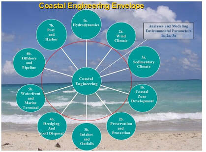 This piece is about the varieties of Coastal Civil Engineering (CCE) works we all see – when visiting seafront to relax, to feel the warmth of ocean in continuous pounding of waves, or when seeing vessels navigating in and out of ports and harbors. These works result from engineering efforts that have three well-known tenets of civil engineering: coastal hydraulic engineering (or simply Coastal Engineering), coastal structural engineering and geotechnical engineering (structural and geotechnical are often lumped together as structures engineering). Coastal hydraulic engineering term is sort of a misnomer – because it not only covers analysis, modeling and determination of hydrodynamic forces caused by water, water level rise and fall, current, wave and bed-level changes – but also includes similar activities due to wind forcing. The combined effects caused by wind and water are known as metocean processes and forces.
Before moving further it is important to build into our concept the extent of geographical area where civil engineering is referred to as CCE (to avoid confusion, CE is reserved to denote Civil Engineering). This area termed as the coastal zone – extends from the inland topographical limit reached by major storm surges and tsunamis to the continental shelf break. Continental shelf mostly of turquoise water, having an average bottom slope of some 1V:100H extends from the shoreline to a seaward line where the slope abruptly dips down into the ocean at about 1V:40H or steeper. This line begins roughly in the region where waves of about ≥ 10 seconds will start feeling the bottom – consequently being subjected to the transformative processes of refraction and shoaling (see Wave Transformation piece on this page). Generally, mariners call the blue ocean beyond continental shelf – high seas. The definitions of inland limit vary among countries – and depend on several criteria such as: technical, legal, administrative, disaster management and hazard insurance – but they all invariably include coastal waterways, river mouths, estuaries and bays. I have discussed many aspects of CCE in different pieces on the NATURE and SCIENCE & TECHNOLOGY (S & T) pages. Thought a piece of introductory nature will complement those. . . . In the US Submerged Land Act (1953) a coastline is defined as: the line of ordinary low water along that portion of the coast which is in direct contact with the open sea and the line marking the seaward limit of inland waters. The same Act defines coastal submerged land under the jurisdiction of coastal States as: navigable waters, and lands beneath, within the boundaries of the respective coastal states out to 3 nautical miles from its coastline. The Outer Continental Shelf Lands Act (OCSLA 1953) defines federal jurisdiction on coastal oceans as: all submerged lands lying seaward of state submerged lands and waters (e.g. outside shelf lands seaward of 3 nautical miles). Perhaps it is useful to add a brief on the legal definition of Maritime Boundary. Part of this brief is based on my 1994 IEB paper: On the Formulation of Coastal Zone Management Plan for Bangladesh. The following definitions of the boundaries are agreed upon by signatory countries (including the land-locked countries which are given the right to claim maritime transport access through their coastal neighbor) at the UN Convention on the Law of the Sea (UNCLOS 1987). It was developed and refined within the framework of the UN – during a period from 1970 to 1984.
. . . There are other names addressing the same problems of CCE but focusing on some particular aspects: like port and harbor engineering, maritime engineering (coined first in European literature), and marine engineering. The last term is loosely applied in civil engineering to describe in-water works – but its root mainly lies in describing mechanical-electrical engineering, navigation and naval architectural aspects of seafaring vessels. Ocean engineering, oceanographical engineering and offshore engineering terms are also used to describe works in coastal and deep waters. Offshore engineering term is primarily applied to describe isolated in-water works in deep water – like oil terminals and marine pipelines. There are many definitions of CCE – different in wording but common in contents. Let us attempt to define it in this piece as: CCE refers to the practice of planning, designing and effects assessment of civil engineering works for the protection and preservation of, and developments (water-front townships and cities, recreation, marine transports and installations, and value-adding improvements) within the coastal zone. The history of CCE is briefly discussed in the Resistance to Flow on this page – it is a fairly new discipline – the official recognition and definition was launched only about 70 years ago – at the First Conference on Coastal Engineering held in Long Beach, California in 1950. Coming back to the definition – one can see that it relies on the understandings of two other terms: civil engineering, and engineering. There are many definitions of these two terms in literature, but I prefer using the following two. According to The National Academy of Engineering and National Research Council: engineering is the study and practice of designing artefacts and processes under the constraints of the laws of nature or science and time, money, available materials, ergonomics (it is the process of designing or arranging workplaces, products and systems to satisfy the needs of people who use them) environmental regulations, manufacturability, and repairability. In NAP #12635 Publication the following texts elucidate the understanding of engineering practices in a very detailed and useful manner (I have rearranged the lines somewhat for clarity). Engineering “habits of mind” (refer to the values, attitudes, and thinking skills associated with engineering; AAAS 1990) align with what many believe are essential skills for citizens in the 21st century. These include: (1) Systems Thinking: systems thinking equips students to recognize essential interconnections in the technological world and to appreciate that systems may have unexpected effects that cannot be predicted from the behavior of individual subsystems; (2) Creativity: creativity is inherent in the engineering design process; (3) Optimism: optimism reflects a world view in which possibilities and opportunities can be found in every challenge and an understanding that every technology can be improved. Engineering is a “team sport”; (4) Collaboration: collaboration leverages the perspectives, knowledge, and capabilities of team members to address a design challenge; (5) Communication: communication is essential to effective collaboration, to understanding the particular wants and needs of a “customer,” and to explaining and justifying the final design solution; and (6) Attention to Ethical Considerations: ethical considerations draw attention to the impacts of engineering on people and the environment; ethical considerations include possible unintended consequences. The 2008 ASCE BOK2 (Civil Engineering Body of Knowledge for the 21st Century, 2nd ed.) defines and elaborates civil engineering as: the profession in which a knowledge of the mathematical and physical sciences gained by study, experience, and practice is applied with judgment to develop ways to utilize, economically, the materials and forces of nature for the progressive well-being of humanity in creating, improving and protecting the environment, in providing the facilities for community living, industry and transportation, and in providing structures for the use of humanity. All these definitions are quite lengthy, but they were developed to cover all different aspects – from scientific, technical, ethical-legal, and societal perspectives. . . . I have written in the Creativity and Due Diligence piece that, CCE as a creative profession has the role . . . in the discipline of civil/hydraulic engineering, applied science provides the baseline knowledge on data and analysis, while technology provides tested products and materials. The role of an engineer is to find solutions to a given problem using resources from these two sources. To do it successfully, it is important for engineers to understand the necessary basics of the S & T. Failing in this matter affects the soundness of an engineer’s judgment. Therefore engineers are part of the S & T endeavors by being intricately involved in the development and progress – sometimes working at the forefront, but most often in the practical applications of science and technological advances to the real-world problems . . . And to accomplish that, engineers by and large, and perhaps more than any other profession – spend a significant portion of their time on computing to create acceptable, defensible and implementable solutions in quantitative terms – using slide rule in earlier times (until about 1970s) to the scientific calculators and personal computers in modern times. Perhaps it is helpful to enumerate some of the sub-disciplines commonly included in the coastal engineering envelope. The first group (a-group) of activities includes those – aimed at establishing critical planning and design conditions and criteria by envisioning the most probable operational and design loading scenarios, uncertainties and risks for various interventions/structures (these structures not only include hard measures of concrete, steel and stones; but also soft structures like beach nourishment and coastal vegetation/tree barriers) based on analysis and modeling of various environmental parameters. This group includes: (1a) hydrodynamics: water level, current, and wave; (2a) wind climate and storms; and (3a) sedimentary climate: coastal geology and sediment transport processes. The second group (b-group) of activities utilizes the first – for planning, designing and assessing the effects and risks of: (1b) coastal zone development and value adding; (2b) coast and shore preservation and protection; (3b) intakes and outfalls; (4b) dredging and spoil disposal; (5b) coastal waterfront and marine terminal structures, including marina; (6b) offshore and pipeline structures; and (7b) port and harbor developments and structures. I have included an image of the coastal envelope showing the discussed disciplines. As indicated earlier, Water Modeling is an integral part of CCE activities. . . . An engineering project starts with a very limited knowledge – starting from that the project moves forward to develop criteria, conditions, specifications, etc. in distinct phases of activities. At the first of three phases – the Conceptual Phase (known as Pre-FEED {Front End Engineering and Design} in Oil and Gas Industries) – starting from scratch problems are defined and the project is visualized, they are then translated into a complete solution package (analysis and design sketches, alternatives, economics, etc) – only at a high level by utilizing available regional and site-specific (mostly unavailable) information. This phase is usually preceded by very high level technical feasibility and economic viability studies. At the next phase – known as the Preliminary Phase (FEED in Oil and Gas Industries) – the conceptual package is critically reviewed, a site-specific information base is established by measurements and modeling, new alternatives are generated, and the conceptual package is revised and updated – but the issued design sketches and specifications are not yet ready for implementation. At the Final or Detailed Phase – a final critical review of the preliminary package is undertaken – updated and refined where necessary, usually no new alternatives are generated – construction, monitoring and supervision methodologies are laid out by detailing each nut & bolt – and the final design sketches and specifications are issued for implementation with the consultant having the additional task of selecting a contractor. The above phases are usually conducted by different engineering consulting firms for better accommodation of talents and ideas, but often the final phase is eliminated entirely for large projects – by combining the final design and construction into a single package. One prominent form of this system is known as the Engineering, Procurement and Construction or EPC method, where the contractor is responsible for the final design, procurement of materials, and delivering the finished functioning product to the client. To assist and oversee the EPC contractor activities – the project owner usually engages a specialist firm known as the Project Management Consultants (PMC). Apart from these, there are many other consulting, contracting and management terms used in different project phases and construction – and they are usually not the same across civil engineering projects – but vary according to types, even from one country to another. . . . A little note on design criteria – they refer to the parameters that must be applied as a minimum for designing project elements; and mostly include: (1) environmental metocean forcing functions, (2) configuration and layout, (3) structural material strength, durability, etc (4) structure-geotechnical, (5) construction and construction foot-prints, (6) operation and maintenance, (7) economics, (8) safety and emergency access, (9) ergonomics, and (10) environmental effects. Some of these criteria are established by scientific and engineering analyses; others come from certified standards and codes; and client and regulatory requirements. Any lapses in not taking proper account of the above criteria constitute a failure. . . . Having clarified the meanings of different terms let us move on to the rest. Let me begin by listing some of the major works identified with coastal engineering. The list is long – I am tempted to provide a brief outline of some important works that are applied worldwide affording developments of manuals, standards and codes (see more in The Grammar of Industrialization):
On Science of Nature Page: Ocean Waves; Sea Level Rise - the Science; Coastal River Delta; Linear Waves; Nonlinear Waves; Spectral Waves; Turbulence; Coastal Water; The Hydraulics of Sediment Transport; Waves - Height, Period and Length; Warming Climate and Entropy; Characterizing Wave Asymmetry On Science & Technology Engineering Page: Common Sense Hydraulics; Uncertainty and Risk; Transformation of Waves; Resistance to Flow; Water Modeling; Sea Level Rise - the Consequences and Adaptation; Tsunami and Tsunami Forces; Storm Surge; The Surf Zone; Wave Forces on Slender Structures; Ship Motion and Mooring Restraints; Wave Structure Interactions & Scour; The World of Numbers and Chances; Managing Coastal Inlets; Propwash; Flood Barrier Systems; Breakwater; Harbor Sedimentation; Uncertainty Propagation in Wave Loadings; Force Fields in a Coastal System; Coastal Ocean Currents off Rivermouths; The Grammar of Industrialization - Standards, Codes and Manual . . . How does one characterize the failure of a structure – like the listed ones? Failures generally fall into 4 basic types: (a) environmental load failure (the cause for this failure is attributed to the exceedence or unexpected occurrence of design loads and loading conditions), (b) functional or ergonomic failure (although the structural integrity remains intact, the structure fails to provide its designed operations, functions or performance), (c) structural failure and (d) geotechnical failure. The last two could have the following 3 causes:
There are many more features of CCE, but for the sake of brevity, I like to stop at this, only to point out one very important aspect. Coastal structures are not like a tall building standing on a dry land – and they should not be treated as such. Because of their exposed location in water or at the water-front, they continuously come under attack by the dynamic and uncertain metocean forcing – from regular to extreme. They must withstand these forces during construction and operational lifetime, as well as face the consequences of uncertain fluid-structure interaction processes, and have to cause minimum impacts on the surrounding environments. Therefore the role of a coastal engineer is very crucial – not only in the establishment of design and operational conditions and criteria, but also during the process of planning, design and construction. Lack of effective coordination, cooperation and concordance among various disciplines – or perhaps in not recognizing the proper roles required of certain disciplines – could lead to earning bad reputation, and to risks of incurring serious economic losses. . . . I like to finish this piece with some lines of poetry written by a seemingly unknown amateur poet, but the poem was made significant by Saint Mother Teresa (1910 – 1997; Nobel Peace Prize 1979; Bharat Ratna 1980; Sainthood 2016) who displayed it in her office. People are illogical, unreasonable and self-centered Love them anyway. . . . Give the world the best you have and you’ll get kicked in the teeth Give the world the best you have anyway. . . . What motivation went into such portrayals of the societies we live in – and the strength and courage the poet was asking for? One can hardly afford not to like the poem – but perhaps more so by a personality none other than Mother Teresa – because it tells all about her life and experience. . . . . . - by Dr. Dilip K. Barua, 5 February 2019 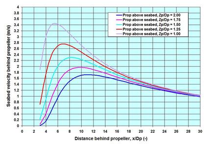 This topic is about the consequences of high turbulence and flow velocity that accompany a fixed-pitch screw propulsion ship. Propwash is the term used to describe the high exit velocity a propeller nozzle generates – and in the context of this piece – it is about the propwash effects on a marine terminal during the berthing and unberthing of a ship. The purpose of generating the high exit velocity by a ship is to cause equivalent forward thrust on it – with Newton’s (Isaac Newton, 1643 - 1727) Third Law of Motion in action. Screw propeller blades are twisted in such a way that a rotating propeller produces a high pressure difference by sucking in waters from one side and discharging them to the other to generate the exit velocity required to push a ship forward. The larger the DWT of a ship (see the Ship Motion and Mooring Restraints piece on this page for DWT) the higher is the requirement of propeller powers. But navy and coast guard vessels requiring high speeds, and Tugs tasked to haul barges or to maneuver large vessels during berthing and unberthing – however small they may be – also need to have high propeller powers. For navy and coast guard vessels – the high speed water-jet propulsion system is more of a requirement because the conventional screw propulsion system would just prove inadequate. Let me share some elements of this important port and maritime engineering topic in simple terms – focusing primarily on propwash and its effects.
. . . Let me begin by focusing on engine thrust that moves a ship ahead. In still ambient water, propeller-induced thrust depends on three important factors – the product of these three describes the efflux – the exiting flux of water from the propeller nozzle. The first is the density of water – which means that with other factors remaining constant – a ship will have somewhat higher thrust in salt water than in fresh water (in addition a ship will feel somewhat lighter in salt water due to enhanced buoyancy). The second most important parameter – is the diameter of the propeller Dp – the thrust is proportional to the square of Dp, implying that it will increase by 4-fold if Dp is changed, let us say, from 1 m to 2 m. Actually, this dependence comes from the equation of the area of a circle – the area being proportional to the square of the diameter. The concept is utilized by encasing the propeller in a duct or short nozzle to obtain more power for the same engine rpm. Despite the engine thrust being highly dependent on the propeller diameter, there is a limit to its maximum size. One of the reasons is that the diameter must scale with the draft of the ship – otherwise a portion of the propeller will surface and rotate in air. But such surfacing cannot be avoided when a ship rides on rough seas with high roll and pitch motions. To describe the third important factor – one needs to take the help of Bernoulli Equation (Daniel Bernoulli, 1700 – 1782). As often pointed out in other pieces, the flow-induced dynamic pressure illustrated by Bernoulli is very important in fluid mechanics – this pressure is proportional to the square of the velocity. Here again, if the velocity is increased, let us say, from 1 m/s to 2 m/s, with other factors remaining constant, the thrust will increase by 4-fold. The exit velocity of an open propeller behaves in a certain way. At a distance of about 0.5*Dp behind the propeller, the exiting jet from an unducted propeller becomes constricted to Do = 0.7*Dp. The maximum jet exit velocity Uo occurs at this location with dissipation taking place further behind. Unlike the other two factors (water density and propeller diameter) – one does not know the jet exit velocity a priori. How to estimate it? To answer this question engineers had to conduct series of lab experiments. Delft Hydraulics took the pioneering role in this regard with HG Blaauw and EJ van de Kaa publishing their paper in 1978 – with more subsequent researches coming from other institutions. Remarkable among these, is a review made by MJ Prosser in 1986. Other notable titles dealing with analysis and design recommendations include: EAU (1996); PIANC (1997, 2002 and 2015), Port Designer’s Handbook: Recommendations and Guidelines (CA Thoresen 2003), Design of Marine Facilities for the Berthing, Mooring and Repair of Vessels (JW Gaithwaite 2004), The Rock Manual (CIRIA 2006), HJ Verheij and C Stolker (2007), and K Römisch and E Schmidt (2009). The first theoretical foundations of the behavior of an expanding jet came from ML Albertson and others (1948) and N Rajaratnam (1976). However despite nearly seven decades of scientific research and engineering, one is tempted to say that propwash and its loading on structures and seabed, and interactions – remain inadequately understood. In the simplest of all the known empirical relations, the exit velocity Uo is described empirically as the product of propeller revolutions per second n, Dp and a thrust coefficient Kt. The dependence on the thrust coefficient is somewhat weak – but a higher pitch (pitch is the distance traveled by a propeller in one complete revolution in no slip condition. Propeller blades are twisted to have a constant pitch from the root at the hub to the tip. The forward travel of a ship is however less than the nominal pitch determined at 0.7*R, R being the propeller radius. The difference is known as the slip. A note on propeller blade numbers – high numbers are usually optimally chosen to minimize vibration and noise.) ensures a higher Kt. Inclusion of Kt makes things somewhat circular – but to go around that, a rough estimate is possible without using Kt – and investigators have developed Kt tables/nomographs for ducted and unducted propellers as a function of the ratio of propeller pitch to its Dp. Another way to determine Uo is to use the applied engine power – and as can be understood, the applied power during berthing and unberthing is usually less than the capacity – varying from some 10% to 35% of the installed capacity. Once Uo is generated, the next important question is what happens to it away from the ship. The afterward behavior of Uo is important because loading on structural elements and seabed depends on it. In the zone of afterward established flow the efflux must mix and dissipate by expanding and entraining the ambient water into the jet boundary. Observations have indicated that in this zone, efflux expands like a cone at an angle of about 12 degrees around the core of maximum velocity. The velocity across the cone decreases from the center following the Gaussian distribution. Along the distance behind the propeller – the whole cone velocity decreases exponentially away from the propeller. At a certain distance behind the propeller, the expanding jet comes in contact with the seabed, causing scour when the sediment pick-up threshold is exceeded. . . . To illustrate the effects of an expanding jet on the seabed, I have included an image as an example – applicable for Dp = 2 m, n = 500 rpm, and Kt = 0.37. The estimated jet exit velocity Uo in this case is 16.2 m/s. The distance behind the propeller x and the height of the propeller axis above the flat seabed Zp are both normalized against Dp. The image shows how the jet velocity at the seabed increases and shifts toward the propeller as Zp decreases. At Zp/Dp = 1.0, the maximum is about 3.4 m/s. The change in Zp could occur, for instance due to the tidal rise and fall of water level, or to a small extent due to loading and unloading of a ship. In the example case, the maximum seabed velocities occurred at a distance x, from 5.3 to 6 times the Zp. The illustrated velocity is a time-averaged quantity – which means that instantaneous turbulence will likely register higher magnitude. Apart from turbulence, the second important one to cause higher velocity – is the effect of rudder behind a single propeller. The rudder splits the jet – and deflects it in one way or another depending on the ship’s heading requirement. At zero rudder deflection, the jet is split into two – one towards the water surface, the other towards the seabed – each making an angle of 12 degrees to the horizontal center – and each spreading at 10 degrees around the core. The implication of rudder deflection (maximum ~ 35 degrees) is that the jet-induced loading and scour phenomena could occur anywhere. The third is the twin-propeller setting with the rudder in the middle. The jets emanating from the two propellers are merged together at some distance (~ 10*Dp) behind the propeller. Unlike the rudder-behind single propeller setting, the deflecting power of the rudder is different, and the seabed velocity enhancement is expected to be less than the rudder-behind-a-single-propeller. However the propellers are often operated independent of each other, making predictions difficult. . . . Some other aspects of ship propulsion systems are also important. There are the thrusters – bow and stern – usually having smaller propellers than the main ones – because of this fact they generate less jet exit velocity. Bow thrusters have mostly a transverse setting – meaning that they draw waters from one side to discharge them to the other – to help sidewise maneuvering of the bow. They mostly have high Zp – thus their effects on seabed are not critical – however the horizontal jets could impinge on quay walls or piles to cause substantial loading. Stern thrusters are mostly omni-directional and are located close to the keel, so that their Zp is rather low. They can play a critical role on causing significant seabed loading and scour. Ship design and propulsion systems are continually evolving (such as podded propulsors, azimuth thrusters and water jets) requiring refinement of known relations, and finding new ones. The consequences of high speed water jet propulsion systems on structures and seabed, open a different dimension to the propwash and associated loading impacts. Apart from these ship-related factors, there are other factors related to the berthing structure – pile orientation, proximity of the sloped bank behind the piles, vertical face sheet-pile walls, etc. All these factors are likely to complicate the jet loading – making the search for critical design conditions difficult – but one thing is certain, it is the potential conditions of repeated loading and incremental progression of damages – that dominate all design and operational considerations. Protecting the seabed against scour-related undermining of the structure foundation for low underkeel clearance setting can be very expensive. For the illustrated case with the maximum seabed velocity of 3.4 m/s, the theoretical median rock diameter is about 0.9 m. Accounting for turbulence factor and other uncertainties associated with rudder, and structural proximity, etc. the required design median rock diameter is likely to be even higher. For such cases, scour protection by bare rock riprap layers can appear impractical. There is an additional danger – it is the sucking-in velocity caused by a propeller with low underkeel clearance, which could suck-in smaller size rocks into the propeller – damaging it. Alternatives such as insitu concrete (such as concrete mattress, grouted rock) and prefabricated mattress (such as concrete block mattress, asphalt mattress, gabion mattress) provide promising options. . . . Let me now briefly focus on another consequence of high jet exit velocity – and it is the drag force the velocity causes on piles supporting a berthing superstructure. To illustrate it simply, suppose there is an offshore marine terminal – a jacket structure standing on 20 m water. Together with dolphins, its purpose is to facilitate berthing, mooring and loading-unloading of oils or gas. A 10-m draft tanker berthing on this facility, likely un-assisted by Tugs, will berth and unberth at the same location repeatedly. If it is located in the Gulf of Mexico, with very little tidal range, it is highly likely that the tanker propeller jets will cause repeated drag loading at the same heights of the jacket-piles. For a case similar like this, the critical aspect is the localized repeated drag forces causing abrasion and bending of the piles. In this situation, the underkeel clearance is likely to be high; therefore any jet-induced seabed loading and scouring effect on the seabed may turn out to be negligible. . . . I like to stop at this – by finishing this piece with a tribute to Stephen Hawking (1942 – 2018) – who despite having debilitating illness did not stop from being active and pursuing his dream for finding a Unified Theory of Everything. He began the 1st paragraph of his book, A Brief History of Time with a little piece of humor: A well-known scientist (some say it was Bertrand Russell, 1872 – 1970) once gave a public lecture on astronomy. He described how the earth orbits around the sun and how the sun, in turn, orbits the centre of a vast collection of stars called our galaxy. At the end of the lecture, a little old lady at the back of the room got up and said: ‘What you have told us is rubbish. The world is really a flat plate supported on the back of a giant tortoise.’ The scientist gave a superior smile before replying, ‘What is the tortoise standing on?’ ‘You’re very clever, young man, very clever,’ said the old lady. ‘But it’s turtles all the way down!’ . . . . . - by Dr. Dilip K. Barua, 9 May 2018 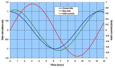 Coastal inlets represent a hydrodynamic connection between two water bodies – the open coastal water on the one hand, and the inland sheltered water body, waterway or lagoon on the other. The name itself suggests that inlets are openings or discontinuities in the shoreline to let oceanic influences such as tide, wave, storm surge and tsunami to propagate inside. They are usually narrow channels that have been historically utilized to install bridges. Another historical significance is that pioneering explorers used the inlets to sail inside into harbors and upriver to discover new lands.
Four different types are usually distinguished – the geological, the hydrological, the human-made and the alluvial-tidal. The first represents a fixed-shore setting that has been formed during the geological processes – straits and many narrows in fjords are of this type. The second represents delta distributaries – the long outlets draining out the river flow into the ocean. In addition to describing them as Estuaries, hydrodynamics and morphological stabilities of this type are better treated as channels – mostly belonging to the deltaic processes discussed in the Coastal River Delta piece on the NATURE page. The third is a dredged-out channel connecting a closed water body to open water. In most cases, the purpose of opening of such an inlet is to develop marinas by facilitating navigation of pleasure boats to and from the marina. The fourth type, also known as the tidal inlet – is the natural response of sandy alluvium to establish a connection between the open coastal water and the inland lagoon. Mostly formed or cut during storm surges, they represent a discontinuity in the barrier island along many littoral shores. These inlets are usually a narrow waterway – its length scaling with width – typically varying from 1 to 5 times the width. Literature is full of materials discussing these types of inlets – their stability, sedimentation, navigation, and technical and economic management issues. . . . Before moving into discussing further, perhaps spending a little time to clarify the term ESTUARY – the hydrological inlet, would be useful.
Moving on – some materials of this piece are based on my Ports2013 paper, presented at the conference in Seattle and published by ASCE: Integrated Modeling and Sedimentation Management: the Case of Salt Ponds Inlet and Harbor in Virginia. This particular inlet was human-made, dredged to develop a marina in parts of the Salt Ponds water body, and connect it to Chesapeake Bay. In this work, sedimentation problems of Salt Ponds Inlet were addressed by coupled numerical modeling {tide + wave + sediment transport + morphology} together with some analytical approaches – among others by comparing wave and tidal powers. Inlet opening, closure or its stability depend on four basic oceanic forcings: (1) regular tidal pumping, (2) wave actions and littoral sand mobilization, (3) episodic but seasonal storm actions, and (4) rarer but powerful tsunami events. The effects of the last two can hardly be overemphasized – in addition to cutting new inlets or closing the existing ones, they impose new boundary conditions that are reworked by the regular forces of tide and wave – to achieve new dynamic equilibrium. Sands are continuously mobilized at the mouth of a tidal inlet by cross-shore and longshore wave actions. If tidal actions do not have the ability to flush out the wave-mobilized sediments, an inlet is doomed to closure. Each year billions of dollars are spent across the world to dredge out sandy shoals of an inlet. The inland parameters influencing an inlet stability is the size of the lagoon, its inter-connection with other systems and the freshwater that drains into the lagoon. The last but not the least is the textural composition of the littoral material, and the amount of sediment loads. Perhaps discussing more of this topic in 3 groups would help streamlining the rest of this piece. . . . Cross-sectional Stability of Tidal Inlets. Three easily identifiable features characterize an alluvial tidal inlet system – the ebb-tidal delta on the ocean end, the flood-tidal delta on the bay end, and a relatively narrow deep inlet channel in-between. There had been considerable interests in the cross-sectional stability of tidal inlets – starting from the beginning of 20th century {to name some investigators: LJ LeConte 1906; MP O’Brien (Morrough Parker O’Brien Jr., 1902 – 1988, considered father of coastal engineering) 1931; FF Escoffier 1940; P Bruun and F Gerritsen 1960; JW Johnson 1973; JT Jerrett 1976; MO Hayes 1980}. In its utmost simplicity, the stability was conceived as a simple behavioral model relating the measured inlet cross-sectional area to the tidal prism – as a central fitting, A = CP^n; with a coefficient C and an exponent n on the tidal prism P. Tidal prism is the volume of water an ocean tide forces through an inlet to fill the inland basin {the prism can either be estimated by integrating, for example the hourly-tidal-flows through an inlet for the window of rising tide – from trough to crest; or as a product of the inland basin area and the tidal height within the basin}. The coefficient and the exponent are adjustable and verifiable parameters and vary from inlets to inlets – but Jarrett’s analyses show that they are in the order of: C = 3.8*10^-5 to 7.5*10^-4; n = 0.86 to 1.03 in SI unit. They were determined {in general, the coefficient is high when the exponent is low; and vice versa} for all the measured jettied and unjettied inlets along the US coast. The simple, yet very insightful model have drawn many follow-up works. It turns out that such a relationship can be established for any tide dominated estuarial channels – e.g. the paper I have presented along with my good friend and mentor Fred Koch in 1986 {Characteristic morphological relationship for tide dominated channels of the lower Meghna estuary, UNESCO, BUET} shows such a possibility. . . . The discussed tidal inlet cross-sectional stability model immediately indicates the following:
. . . Inlet-Bay Hydraulics. Despite providing a first-order understanding of the inlet stability and more, the reality of the problem is much more complex than the simple inlet cross-sectional stability formula. One way to appreciate this is to examine the one-dimensional Saint-Venant hydrodynamic equation applicable in long inlets (French mathematician Adhémar Jean Claude Barré de Saint-Venant, 1797 – 1886). This equation is only solvable by numerical modeling, but an analytical solution to the problem was offered by GH Keulegan (1951) and DB King (1974). This can be very useful to have an improved impression of the inlet current and the bay tidal response. To illustrate its application, an image is included showing the ocean tide, bay tide and cross-sectional current. It is applicable for: inlet length 5 km; inlet width 3 km; inlet depth 15 m; bay depth 10 m; bay area 300 million square meter; tidal period 12.42 hours; and tidal range 2 m. In this particular example, the bay tide is slightly amplified and lags behind the ocean tide. The illustrated example is only good for preliminary assessment. To better understand the complicated inlet-system processes – a coupled shallow-water numerical model may prove to be the best recourse – like the one described in my Ports2013 paper. Since opening of the Salt Ponds Inlet in 1979, the City of Hampton is required to dredge the inlet every 2 to 3 years to maintain its navigability. This frequency of recurring dredging is quite a burden and has not decreased despite the construction of jetties at the inlet mouth. Presented as a comparison of tide and wave powers – it turns out the tidal prism of the inlet is quite inadequate to flush out the sands mobilized by wave actions – active in the Chesapeake Bay. . . . Managing Tidal Inlets on Littoral Shores. The problem of such inlets primarily hinges upon keeping them functional, open and navigable – this is necessary because most large inlets cater to the needs of ports, harbors and marinas – for in-and-out sailing of different types of vessels. What issues must one look for sound management of such an inlet? Let me try to highlight some briefly.
. . . . . - by Dr. Dilip K. Barua, 16 March 2018 |
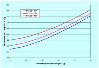
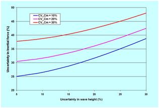
 RSS Feed
