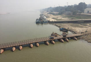
 No man ever steps in the same river twice, for it is not the same river and he is not the same man. What a piece of wisdom from the Greek Philosopher Heraclitus (535 – 475 BCE) on the facts of Nature, life and society - the reality of impermanence (Gautama Buddha - The Tathagata, 624 – 544 BCE) that defines the ever changing fluxes of mind and matter and all things that surround us (impermanence does not connote, for example, that a relationship is not supposed to last, but that the nature of relationship does not remain the same over time). Apart from some obvious reasons – humans had been attracted to rivers since time immemorial, feeling and witnessing their vibrating energy and transformative changes – rich with the messages of the realities of life. This piece is not about this reality – but the reality of a different sort – the macro-scale processes that define a river. And understanding these processes equip us to better manage a river.
These are the aspects we all know about yet do not pay adequate attention to – we tend to think of those aspects so guaranteed that we often fail to take proper account of them while planning catchment and river-bank developments, flow-interventions, or while dumping materials of all sorts into them. These are the basin-wide factors that control the birth and flow of a river defining its characteristics, and the functions it shoulders on its journey. The factors and functions are unique to each river – and define the characteristic regime of a river system. A river is better understood as a system comprising of the tributaries that contribute to its load; the distributaries that carry part of the load; the floodplains that alleviate its burden by functioning as a storage basin, and slowly releasing the flood water; and the delta it builds as it debouches into open water. But while one talks about the basin-wide factors – encompassing the catchment area from the headwaters to the base level at lake or sea – a river has also distinctive reach-wise factors of geology, geography, hydrology and hydraulics. People often see a river analogous to life – birth and infancy at the source, energetic youth at the steep terrain, broad and mature adult at the flat landscape, and demise at the base level. And since the geologic past, the river has been giving away the resources (hazardous when angry – flooding its basin) it carries – to quench thirst, to help cultivate lands, to build navigational trade networks, townships, cities and civilizations. No wonder – philosophy, poetry, fictions and religions are full of inspiring materials on river – with some attributing divinity to it. . . . With these paragraphs of introduction let me move on to the core materials of this piece. For simplicity and importance, I will primarily focus on alluvial rivers (a river that constantly changes and defines its own deformable granular bed and planform depending on the volume of water it carries and the magnitude and type of sediments it transports). The discussed aspects are based on my short river experience and three of my published papers:
. . . What are the environmental controls of a river – that define its unique characteristics (for example, those responsible for distinguishing the Mississippi River from the Ganges-Brahmaputra system)? A river is the dynamic response of the earth’s surface to the draining of accumulated water mass. The accumulated water mass contributed by precipitation, snow and glacier melt is collected by numerous streams and gullies – all feeding to the development of a river. Rivers are also a showcase of annual hydrologic wave – the seasonal river discharge; but without the usual reversal of flow – rather with the wave-type fall-rise-fall-rise water level stages. As observed in the Bangladesh Reach of the Ganges River (my 1995 IEB paper), the river flows can be characterized in terms of a Seasonality Index (this parameter defines the river regime and is very useful to distinguish the hydrologic characteristics of one river from another) – indicating a rather steeper slope during the rising phase than the falling period. The implication of such an asymmetry lies in the existence of the so-called hysteresis or incoherence in the relationship between river stage and discharge – and between the discharge and sediment transport. The dynamic behavior of a river represents an interactive process-response system driven by universal physical laws - but the actions and reactions take place within the boundary conditions or environmental controls where it belongs. What are these? The list is simple – (1) climate, (2) catchment basin size, (3) basin relief or slope, (4) type and extent of basin Natural vegetation, (5) basin lithology defining the soil material characteristics, (6) anthropogenic factors, (7) frequency and magnitude of episodic events, (8) base level or sea level changes, and (9) earth’s rotation. The last factor – the effect of earth’s rotation is important for large rivers. While the list is simple, the controlling influences are not – because each of these factors has different variability and time-scales of change – the characteristic signature depending on the geographical location where the river belongs. And any change of these factors invokes a response from the river – the response depending on the magnitude, intensity and frequency of changes or modifications. What are the responses? An alluvial river response to the above driving conditions can be thought of as comprising two categories. The first is the Fluvial Loading – water discharge, sediment transport, and sediment caliber (the sizes and types of sediments a river transports). The second is the Fluvial Geomorphology – width, depth, slope, and planform (such as meandering or braiding type). Both of these two categories are conditioned by environmental controls – with the fluvial loading acting as the imposed processes on the fluvial geomorphology. Together they represent an interactive process-response system that aims to attain dynamic equilibrium in time. Discussing all the factors can be very elaborate, let me focus on two important ones:
At the outset it is important to make a distinction between resource and hazard. This distinction depends on defining a threshold for a particular phenomenon. The simplest of this is the flood level that one hears most often. The defined threshold helps planners and engineers to classify a river stage, whether or not it is at danger level or at tolerable level. When the threshold is exceeded, the water as a resource becomes hazardous. Another simple example is the much talked about proliferation of carp fish in the Mississippi River. It was a resource in small numbers, but as this invasive species overwhelmed others, the same fish has become hazardous. . . . The functions can be thought of as comprising four important broad groups: (1) biotic, (2) abiotic, (3) functional use, and (4) consumptive or diverted use. The biotic function is the sustenance of flora and fauna that thrive in a river basin. The most important biotic function is the fresh and brackish-water fish resources a river produces and sustains. Any change in the discharge volume, water temperature, salinity regime affects this important resource – most humans rely on for nutrition. A measure of the biotic function often relies on the level of dissolved oxygen (DO) and biological oxygen demand (BOD). Here again a threshold needs to be defined for a particular species – a higher BOD than the available DO can turn the same water from a resource to a hazardous one. In addition to dissolved pollutants that affect water oxygen level, floating non bio-degradable debris limits the recreational functions of a river. The abiotic functions can be elaborated as: (a) drainage of surface run-off, (b) drainage of subsurface flows, (c) sustaining geomorphologic equilibrium, (d) land building in the deltaic reaches, and (e) preventing salt-water intrusion in estuaries. Functional use accounts for navigation, open-water fisheries and fish migration, and recreation. The biotic, abiotic and the functional use are essential river functions – let us say duties, a river is tasked to do. The extent of these tasks defines a river. Any unthoughtful development or intervention that does not give importance to its functions can jeopardize the long-term health and equilibrium processes of a river and its riparian areas. Consumptive or diverted use – on the other hand accounts for net loss of river-water. They include: (1) domestic/municipal, (2) agricultural, (3) industrial – hydropower and cooling, (4) culture-fisheries, and (5) inter-basin water transfer. How much water a river afford to lose without compromising its essential functions? The question does not have easy answers – and definitely arises again and again when dams and inter-basin water transfer are planned. There exist many conflicts on the equitable sharing of waters by co-riparian states and countries. But when such plans are implemented, the old river ceases to exist – and its regime and basin characteristics are changed for ever. Most rivers around the world have lost their past regimes or characteristics because of extensive damming, dikes and urban developments. Let me now attempt to elaborate the functions of a river – but for the sake of brevity focusing only on two of them:
An equitable trade-off is often not easy to find without impacting one or the other – the goal then is to search for ways to minimize impacts. It further entails that – water and sediment management of a river – should be based on a holistic view of the entire system of river network by encompassing all the forces and processes – beginning right in the upper catchments – to the lower floodplain – down to the delta. There are many instances that suggest that traditional methods of farming, land-use and water use – were effective and respectful to the sustenance of Nature – and the habitat of multiple flora and fauna it accommodates. Therefore, it is only prudent that – conceiving and planning a development project must pay diligent heed to all different interdependent environmental aspects. A solution must strive to accommodate traditional practices into the modern engineering methods – to minimize unwanted and adverse effects and impacts on the system and on stake-holders – both in time and space. . . . Like the energy of a river, let the vitality of life flow into the New Year and to all years to come. . . . . . - by Dr. Dilip K. Barua, 26 December 2018
0 Comments
 Waves were the focus of discussions in at least 5 pieces on this NATURE page, and in 1 and more pieces on the SCIENCE & TECHNOLOGY page. I am tempted to add another piece – because understanding of the wave processes and their loadings and other effects on structures and seabed is very important – not only for coastal/hydraulic civil engineers but also for all. We have discussed in some other pieces that wave is the fundamental mechanism how energy is transformed and transported – in fluid flows, in climatic patterns and changes, in electro-magnetism, and in societal behaviors of plants and animals including humans. Sometimes when the wave length is too long – for example, in seasonal river flows which we tend not to consider as a wave – but the long-term behavior of a river and its alluvial morphology is better understood if the river seasonality is properly characterized.
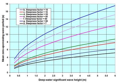
This piece is about 3 integral parameters of waves – the height (simply the height between successive crests and troughs), the period (simply the time lapse between two successive crests or troughs) and the length (simply the distance traveled by two successive crests or troughs), and the inter-relationships among them. These three parameters are integral – because they convey no indication of the shape of a wave – its symmetry or asymmetry. We have discussed in other pieces {Ocean Waves; Linear Waves; Nonlinear Waves; Spectral Waves; and Transformation of Waves} that Natural waves are irregular, random and spectromatic – and that they can be approximated as linear or nonlinear based on a single parameter – the Ursell Number (Fritz Joseph Ursell, 1923 – 2012). This parameter describes a threshold combining the two ratios H/d and d/L, and is given by U = HL^2/d^3 {H = wave height; d = water depth; L = local wave length; and T = wave period. For spectral waves, Hs = significant wave height, average of the highest 1/3rd of waves; Tp = wave period corresponding to the peak spectral energy}. It turns out that for all practical purposes, waves can be assumed to be symmetric or linear, when U is equal to or less than 5.0. . . . Perhaps it is helpful to begin with some principles of monochromatic wave as we move on to discussing Natural waves. Among the parameters, the wave period T and the wave length L are uniquely related via the celerity C – the propagation speed of the wave energy; L being the product of C and T. In deep-water with d/L ≥ 0.5, waves do not see the depth; therefore C is solely a function of T, with L becoming a function of T^2. One implication of this dependence becomes immediately clear – it is the decomposition of a spectromatic wave composite into its component frequencies – the longer period component having higher C, dispersing out from the shorter ones. This is how one explains the incoming swells arriving first on shores – as the precursor of a storm. With decreasing water depth, starting at d/L ≈ 0.05, wave attains the characteristic of a long wave or shallow-water wave, and C becomes a sole function of depth d. For C to go through the transformation (from independence to the dependence on depth), the wave period T must remain constant. In a chapter, Small Amplitude Wave Theory (Estuary and Coastline Hydrodynamics, ed. AT Ippen, McGraw-Hill, 1966), PS Eagleson and RG Dean demonstrated the necessity for constancy of wave period by considering a simple harmonic wave train as it moves from deep to shallow water. It is simply argued from the principle of the conservation of the number of waves propagating from one section to the next, that – it is either the wave period or the length that must change to ensure the continuity – since the wave length changes following the changing C, the period must remain constant. There is a transitional region between the deep (d/L ≤ 0.5) and shallow waters (d/L ≥ 0.05) where C depends on both T and d. These dependences make it difficult to determine L explicitly. In modern times with digital computation, that difficulty has been overcome. But a simple relation proposed by HN Hunt in 1979 yields values that are surprisingly close to the exact L. There is another aspect of wave length: what we have discussed so far is the linear wave length for U ≤ 5.0; in shallower water with higher U, the actual wave length (nonlinear) becomes longer, differing from L – the difference becomes wider as the wave propagates to increasingly shallow water. For example, for a 2-m high 8-s wave, at U ≈ 30.0, L = 57.5 m, Stokes 5th order L_5th = 60.2 m, the Cnoidal L_cnoidal = 68.9 m. While the relationship between wave period and length is simple, the same between wave height and period is not straightforward. The reason is that wave heights can be associated with a wide range of periods – as evident from the scatter diagrams one sees in observed Natural waves. They usually vary according to wave steepness – the steepness being the ratio of H/L – from (1/7 ≈ 0.143) to (1/80 ≈ 0.013). The first is the limiting high steepness – at and above which a wave cannot sustain itself and must break (the criterion proposed by R Miche 1944, 1951). The second represents roughly the limit of observed waves dominated by long-period swells in coastal oceans. . . . To demonstrate the wave height-period association of spectromatic waves, I have included an image showing the relationships between mean zero up-crossing wave period Tz and deep-water Hs – based on a relation proposed in my 2015 World Scientific paper: Longshore Sand Transport – An Examination of Methods and Associated Uncertainties. The family of lines for different steepness factors (reciprocal of steepness) shows the relationship from high steepness (line a) at the bottom to the low at the top (line g). For 1-m wave height, the period-envelop varies from 2.12 s to 7.16 s; for a 6-m high wave it is from 5.19 s to 17.53 s. What is the working relationship between Tz and Tp – the wave period of practical interest? Following CL Bretschneider (1969) – who has shown that, the square of the wave period follows the asymmetric Rayleigh distribution – the peak spectral period Tp ≈ 1.41Tz. Unlike the constancy of a single monochromatic wave period, Tp is not something that remains constant for a wave group – it evolves as the energy is transferred and redistributed within the group due to non-linear wave-to-wave interactions and other transformational processes – therefore the downstream peak spectral wave period is not same as the upstream. The identification of the physics of this interaction process is fairly new and has been attributed to the contributions made by Hasselmann and others (1985). Here are some explanations of the wave-to-wave interactions.
It is time to wrap this piece by exploring the mind of Spanish painter and sculptor Salvador Dali (1904 – 1989) . . . Have no fear of perfection – you’ll never reach it . . . Professional context? Imperfection – but of the learned mind to be meaningful and justifiable. . . . . . - by Dr. Dilip K. Barua, 20 June 2018 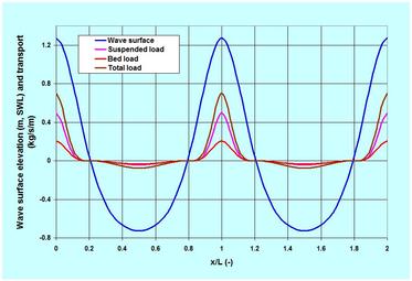 When I started writing this piece, I thought of a title like: The Hydraulics of Sediment Motion. Well this would not have been right – would it? The reason is that sediments need energy from water motion – they do not have any to propel themselves. They need local hydrodynamic energy to be picked up from the bed – to be transported hopping up and down near the bed – and to be carried while in suspension in the water column. Because of this necessity, sediment transport processes are alternatively referred to as sediment load dynamics. The loads are carried by the water motion as long as the local transport power exceeds the downward gravitational pull acting on the sediment particles.
Before moving further one needs to clarify a distinction however. This distinction between non-cohesive and cohesive sediments and transports is based on the relative dominance of gravitational and electrochemical forces. The non-cohesive texture is dominated by individual sand grains (> 0.063 mm) – their settling and transport are controlled by gravity. For silt (0.063 mm > silt > 0.004 mm) and clay (< 0.004 mm) sized particles, on the other hand, the electrochemical processes (function of mineralogy and water chemistry – salinity and temperature) of aggregation and flocculation play a dominant role in binding individual particles loosely together. My own experiments {Discussion of ‘Management of Fluid Mud in Estuaries, Bays, and Lakes. I: Present State of Understanding on Character and Behavior’ ASCE Journal of Hydraulic Engineering, 2008} throw some insights on this. Analysis of mud samples (median diameter varying from 0.006 mm to 0.011 mm) consisting of 14.9% to 34.1% clay content (characterized by clay-size mineralogy: 52% illite, 23% kaolinite, 15% smectite, and 10% others) shows exponentially decreasing suspended sediment concentration with increasing salinity – an indication of enhanced salinity-induced flocculation and settling. Once deposited, the cohesive sediments form a loosely packed easily erodible fluid-mud layer, which becomes hard mud through the slow processes of consolidation. The transport of cohesive sediments is often termed as wash load transport – as opposed to bed-material transport – with the arguments that their concentration and transport are independent of local hydrodynamics and bed-material composition. As a blanket classification, all silt and clay sized particles (< 0.063 mm) are considered as wash load. In one of my IEB papers (Sediment Transport in Suspension: an Examination of the Difference between Bed-material Load and Wash Load, IEB 1995), I argued against this blanket classification and showed from field measurements that the classification should instead be based on local hydrodynamic energy criteria proposed by Vlugter (1941) and Bagnold (1962). . . . This piece is about non-cohesive sediment transport dynamics in alluvial coastal waters. This type of transport is notoriously erratic due to the continuous interactions between gravity, and flow turbulence – more vigorous within the boundary layer close to the bed than in layers upward in the water column (see the Turbulence piece on this page and my IAHR paper published by Taylor & Francis – where it is shown that bed-turbulence reaches peak at 5% to 10% of depth above the bed). The transport in coastal waters can be distinguished as two basic types: the transport within the wave breaking surf zone is highly driven by breaking wave turbulence – liquefied and suspended by turbulence, the sediments are transported in this zone by longshore and cross-shore currents – by undertow offshore currents, and by longshore currents generated by obliquely breaking waves. See more in The Surf Zone. Outside the surf zone, sediment transport dynamics are dominated by processes similar to steady currents – but in somewhat different fashions accounting for nearbed wave orbital velocity, friction factor, and other currents generated by tide, tsunami and storm surge. The transports within the surf zone are not covered in this piece – hope to come back to this at some other time. This piece is on bed-material transport and processes outside the surf zone. There are colossal amount of literature on bed-material sediment transports – to the extent of some confusion. The reason for so much attention and investments is that the sedimentation management and engineering comprise a very complicated problem – not only because of the complicated theories and relations, but also because of the real-world hydrodynamic actions in varied frequencies and directions and corresponding responses of the alluvial seabed. The result is that although there are general agreements on the nature of dependent variables, very few relations agree in terms of inter-relationships, and in predictions of transport quantities. So it is no surprising that the disagreement in predicted transports can vary by as much as ± 100%. Let us attempt to understand all this in a nutshell – and as we move along, references used for this piece will come to light – including some of my published works. . . . What must one look for in studying sediment transport dynamics? Here is a brief outline.
. . . Nearbed Fluid Forcing and Bed Resistance. To describe this aspect of the transport dynamics, I will mainly use materials from my 2017 published chapter in the Encyclopedia of Coastal Science (Seabed Roughness of Coastal Waters). In an oscillatory environment of coastal waters, the nearbed fluid forcing or bed-shear stress is formulated in terms of the quadratic friction law, which is rooted in Bernoulli (Daniel Bernoulli, 1700 – 1782) theorem. The bed resistance in the friction law is expressed in terms of a drag coefficient (or its equivalent: Chezy C, Manning n and Darcy-Weisbach f) in currents, and a friction factor (fw) in waves – its value depending on the seabed sediment texture and bedforms. The quadratic friction law says that the bed-shear stress is the product of a friction factor, fluid density and the nearbed orbital velocity squared. As an example: for a low-steepness, 2-meter high 12-second wave (wave steepness = 0.017) at 10 meter water depth on 0.5 mm coarse-sand seabed, the peak wave friction factor is 0.0089 – exerting an equivalent peak wave-forced bed-shear velocity of 0.079 m/s. As the Ursell Number (U = 26.8) is very high – Stokes 5th order nonlinear wave theory is applied for the estimates. . . . Sediment Pick-up Threshold. The threshold dynamics can simply be thought of like this: while a particle lying on the seabed is subjected to the fluid forces of drag and lift, the weight of the particle and its position (frictional resistance) within the pack resist these forces. In currents, the pioneering experimental work was done by Shields (1936) – his graphical solution provides the threshold Shields Parameter as a function of particle Reynolds Number. As an attempt to make life easier for digital computation, Soulsby (1997) proposed an adaptation of this relation that helps one to estimate threshold depth-averaged velocity as a function of Particle Parameter. For waves, the estimation methods of the threshold are not very well-established. For the 0.5 mm seabed and the example wave, use of a relation proposed by Komar and Millar (1974) shows the peak threshold nearbed orbital velocity as 0.17 m/s. Comparatively, the exerted nearbed orbital velocities by the wave vary from the offshore -0.63 m/s to the onshore 1.2 m/s, passing through the zeros in-between. This indicates that there would be no motions of particles during some brief periods of the wave-cycle. . . . Suspension Criteria and Profile. The Suspension Number discussed earlier tells that particles remain in suspension when the bed-shear velocity is equal to or exceeds the particle settling velocity {also my paper: Discussion of ‘Simple Formula to Estimate Settling Velocity of Natural Sediments’ ASCE Jr of Waterway, Port, Coastal and Ocean Engg, 2004}. The same seabed sediment particle of 0.5 mm having a settling velocity of 6.1 cm/s (according to Rubey 1933), would require to have a fluid forcing bed-shear velocity larger than this. For the example wave, the equivalent peak bed-shear velocity is 7.9 cm/s yielding a Suspension Number of 1.3. The exercise indicates that the particles will remain suspended around the peak, but will tend to fall toward the bed during other phases of the wave-cycle. Once suspended, the nature of the suspension profile (a profile from a certain value at the surface to an exponentially increasing concentration near to the bed) will depend on the value of Rouse Number. The peak Rouse Number for the example wave, and the bed-material size is 1.92. Here again, one should note that this number varies over the wave cycle – which means that the fate of a suspended particle whether dropping on to the bed or remaining suspended, would depend on the particle’s position in the water column – the higher is its original position in the water column the lower is its chance of reaching the bed. The integration of the product of suspension and velocity profiles over the water depth (from a certain height above the bed) yields the suspended load transport. Such integrations are affected by some errors, however {my paper: Discussion of ‘Field Techniques for Suspended-sediment Measurement’, ASCE Journal of Hydraulic Engineering, 2001}. This happens because of the practical constraints of measurements in discrete intervals of space and time. . . . Sediment Transport Rate. Traditionally the derivations of sediment transport predictors are based on two approaches. The first is based on measurements that attempt to correlate the transport rate to some known hydraulic parameters. The second is based on laboratory experiments and scale-modeling tests relying on dimensional analysis of variables. These two approaches – often miss and obscure a very import aspect of sediment transport hydraulics – and it is the physics. Physics has the rare capability of enhancing one’s capability of understanding very complex problems. Help in this regard came from an unusual source – a World War veteran, Ralph Alger Bagnold (1896 – 1990). His ground breaking book, The Physics of Blown Sand and Desert Dunes (1941) proposed a relation of sand transport that depended on the fluid power. The fluid power is proportional to velocity, U raised to the power 3, U^3. It really makes sense because the forcing on the bed (bed-shear stress) to dislodge a particle is proportional to U^2. The transport flux or the power to transport the dislodged particles then becomes proportional to U^3. In a 42-page paper (US Geological Survey Professional Paper 422-I, 1966), An Approach to the Sediment Transport Problem From General Physics, Bagnold proposed the same approach to formulate the bed load and suspended load transports in steady water-current environments. His approach has been refined and reworked by many investigators – but the 1981 paper by JA Bailard, An Energetics Total Load Sediment Transport Model for Plane Sloping Beach made significant contributions – by adapting the Bagnold relation for oscillatory environments of waves. Among others, Bailard took the advantage of quadratic friction law to define the bed shear stress. His proposed relation popularly known as Bailard-Bagnold sediment transport formula is gaining popularity in recent times. The formula reflects bed load transport as proportional to U^3, and the suspended load transport requiring more energy to overcome the settling velocity as proportional to U^4. In this piece, I will demonstrate the application of this relation for the example wave, to show the cross-shore sediment transport outside the surf zone where wave asymmetry or nonlinearity plays a significant role. To illustrate the application of this method – I have included an image showing the wave surface of the example 2-meter high 12-second wave, and instantaneous cross-shore bed, suspended and total load transports for 2-wave cycles. It is assumed that the wave approaches the shore directly with its crest parallel to the shore. At 10-meter water depth on a seabed slope of 1/50 and a median sand particle diameter of 0.5 mm, the wave becomes asymmetric or nonlinear (Ursell Number U = 26.8) indicating the heightening of the crest and flattening of the trough. As expected, the image shows high onshore transports under the crest (maximum onshore nearbed orbital velocity 1.19 m/s) and low offshore under the trough (maximum offshore nearbed orbital velocity -0.63 m/s). In terms of the total load transport per meter parallel to the shore – the maximum onshore is 0.71 kg/s, and the maximum offshore is -0.07 kg/s – with the net onshore transport during one wave cycle as 2.13 kg. The ratios of suspended load to bed load vary from 0.01 to 2.4. If the period of the 2-meter wave is reduced to 5-second (the wave steepness increases to 0.06), linear wave theory applies (U = 2.7), and the net onshore transport reduces to 0.12 kg per meter parallel to the shore. The period-effect of nonlinearity and high net onshore transport is one simple example of beach build-up that happens in most beaches during the summer-time season of low-steepness swells. Like many other sediment transport predictors, Bailard-Bagnold formula is not without limitations. To allow some flexibility in this regard, the formula allows it to calibrate to measurements by two adjustments – the bed-load and the suspended load efficiency factors. Like the colossal amount of literature in sediment dynamics, this piece turned out to be another long piece in the WIDECANVAS. Well, I suppose one needs to make things clear one is attempting to explain. Let me finish this piece with a quote from Albert Einstein (1879 – 1955), who reportedly asked his son Hans Einstein, Why is it that you wish to study something so complicated? Hans Einstein indeed saw the complicated sediment transport problem more profoundly – in terms of probability theory – proposing his own probabilistic sediment transport formula (Einstein 1950). . . . . . - by Dr. Dilip K. Barua, 15 November 2017 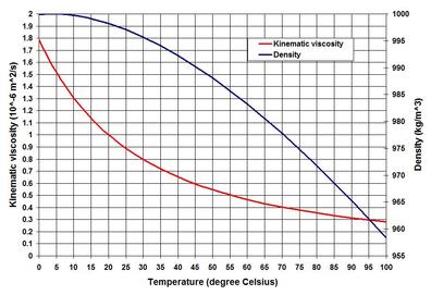 The title of this piece has a very broad range of subtopics – some of which have already been discussed previously on this website. In this piece let us talk about some properties of coastal water – the properties that appear in most methods and equations of coastal hydraulic science and engineering – as referred to in some pieces on the NATURE and SCIENCE & TECHNOLOGY pages. In brief, these properties include the mass of coastal water, its resistance to sliding motion, and its resistance to compression. These three properties – the seawater equation of state, viscosity and compressibility are most interesting to physicists and engineers.
When one thinks of coastal water – some common views immediately appear – close to the sources of freshwater such as river mouths and estuaries it is brackish (diluted mix of fresh and salt water) – further away from the source it is close to seawater salinity. It is mostly mixed in the top surface layer and in waters where the basin aspect ratio (ratio of vertical and horizontal dimensions) is very low, but is stratified to some degree in basins of high aspect ratio. The stratification – in terms of both temperature and salinity – in sharp lines of distinctions is known as thermocline and halocline, respectively. I have touched upon the stability of stratification in the Turbulence piece – but there are more on the topic – hope to come back to that at some other time. . . . Before going further I am tempted to make one important observation. This is the fact that the variability of these parameters in coastal waters is so negligible that coastal engineering literature has very little room discussing them. In the Delft lectures of coastal engineering, we were told that one of the key words for practicing engineers was approximation – approximation! In the coastal and estuarine oceanographic lectures at the USC, professors did not forget to mention that mistakes in the use of different but close numbers in density and viscosity were very negligible. Although approximation is one of the major techniques in every branch of social and Natural sciences, it has a particular significance to the practicing engineers because they often find comfort in hanging on to a certain number – reasonable enough to justify and safe enough for their problems. Despite such a view, unless one understands the science of seawater physical properties, it is often impossible for him or her to overcome the feeling of uncertainty. This certainly applies to the blue-water oceanographic investigators who cannot afford to ignore the variability of seawater properties, because they deal with depth scales in the order of 100s of meters and length scales in the order of kilometers. . . . The 2010 UNESCO document on seawater thermodynamics is one of the most extensive recent treatises on the seawater equation of state. It expresses seawater density as a function of salinity, temperature and pressure. The density (mass per unit volume) is also often expressed as specific volume (reciprocal of density) and specific gravity (the ratio of density of any matter and the density of freshwater at standard temperature of 4 degree Celsius) – is not the unit of force like the specific weight (density times the acceleration due to gravity). In oceanographic literature, the seawater density is usually shown as an anomaly – as sigma-t. This anomaly is just a way of expressing things for convenience, and is nothing but the density of seawater in excess of the freshwater density of 1000 kilogram per cubic meter of volume (kg/m^3). Most old oceanographic literature used to present the complicated equation of state as a graphical method until the UNESCO elaboration was published. For all practical purposes, the polynomial UNESCO method is approximated as a linear equation that comes with an error of ± 0.5 kg/m^3. Among the three independent variables, pressure has the least influence on seawater density – which in essence tells that water is very negligibly compressible. The fluid pressures are usually measured in bars (1 bar equals to a pressure of 100 kiloPascal or kPa) – the atmospheric pressure on the Earth’s surface is 1000 millibar or 1 bar; and 1 meter of water exerts a pressure of 1 decibar (=10 kPa; this is the usual unit used for water pressure). Other influences remaining constant, the water density increases by only 1 kg/m^3 in every 200 meter (or 200 decibar) of depth increase. The water density has a strange relationship to temperature – the freshwater density is the highest 1000 kg/m^3 at a temperature of 4 degree Celsius – but decreases in both higher and lower temperatures from this threshold value (note that the mean ocean temperature is about 3.5 degree Celsius). As a rule of thumb, water density decreases by 1 kg/m^3 for every 5 degree Celsius rise of water temperature. But as shown in the image, the relationship between water density and temperature is far from linear – so is viscosity. I will come back to viscosity later, before that let me elaborate some other aspects of seawater salinity. Among the three parameters, salinity affects the seawater density more than any other. It was used to be measured as a gram of salt in one kilogram of solution, and presented in units of parts per thousand (ppt or o/oo). Salinity is now referred to as Sp on the unit-less Practical Salinity Scale or PSS-78 following the 1978 UNESCO definition. The PSS is defined as the ratio of seawater conductivity to the conductivity of standard KCL solution. For all practical purposes the two systems – ppt and Sp are equivalent, but Sp applies in the range from 2 to 42. The average seawater salinity is about 35 Sp – the highest ocean water salinity is concentrated in the sub-tropical gyre region between 20 and 30 degree North and South latitudes where rainfall is the lowest. Some orders of magnitude seawater density for salinity? For 5, 10, 20, 30 and 35 Sp, the corresponding densities are 1003.6, 1007.5, 1015.3, 1023.1 and 1027.0 kg/m^3 in 1-meter depth of water at a temperature of 10 degree Celsius. For most coastal engineering problems, a density of 1025 kg/m^3 is applied. If one uses 1000 kg/m^3 instead of 1025 kg/m^3, the incurred error is only 2.5%. . . . Let us now turn our attention to viscosity (a term reciprocal to fluidity). This water characteristic – the molecular viscosity (as opposed to the eddy viscosity discussed in the Turbulence piece) is a dynamic property – it is the resistance of water to shearing or sliding motion. It was formulated by none other than Newton (Isaac Newton, 1643 – 1727) as a proportionality coefficient in the relation between shear stress and shearing rate of deformation. The fluids such as water that have a constant proportionality coefficient are known as the Newtonian fluids. The coefficient is known as the dynamic viscosity coefficient – a product of density and kinematic viscosity. While viscosity is a function of density, in many applications it appears as the kinematic viscosity – as a matter of convenience in managing equation terms in the cases of homogenous water of equal density. In some other cases of fluid mechanics problems, the effect of viscosity is so low that the term is neglected all-together, giving rise to the term inviscid fluid or ideal fluid. The included image shows the kinematic viscosity as a function of temperature. The kinematic viscosity of freshwater at 20 degree Celsius is about 1*10^-6 meter squared per second – the air viscosity is about 1/50th of water. Let us now turn our attention to the last term – the compressibility. This term refers to resistance to change in volume in response to change in pressure. It is reciprocal to the volume or bulk modulus of elasticity (BME) – a coefficient defining the change in pressure in response to change in volume. The definition of BME originates from the Hooke’s (English mathematician Robert Hooke, 1635 – 1703) Law of stress and strain; and Young’s (English scientist Thomas Young, 1773 – 1829) modulus of elasticity. The water BME increases with high pressure but has a strange relationship with temperature – it is highest at 50 degree Celsius – decreasing in both higher and lower temperatures. The higher the value of the BME, the lower is the compressibility. The typical water BME is 2.2 million kPa. Such a high BME means that water needs very high pressure to change in volume – or to be compressible – leading to the common assumption that water is incompressible. One of the implications of very low compressibility of water is that the speed of sound is very high in water – some 1500 meter per second – about 4 to 5 times faster than the speed in air. The speed of sound increases as water temperature, salinity and depth are increased. . . . Well there is much more on water properties than what are discussed. For now, let us leave it at this – on this wonder substance called water – a breeder and sustainer of life. Let us finish this piece with a word of wisdom from Lao Tzu: nothing is softer or more flexible than water, yet nothing can resist it. . . . . . - by Dr. Dilip K. Barua, 1 December 2016 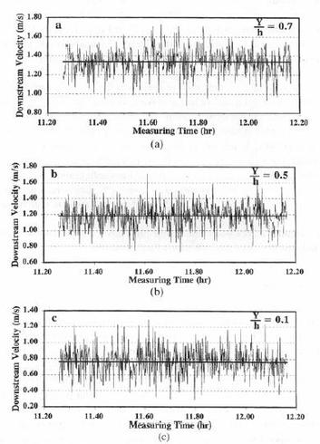 In this piece let us talk about another important phenomenon in the field of fluid mechanics – turbulence – focusing primarily on its processes and characteristics. To do this I will take help from my 1998 Journal of Hydraulic Research paper: Some aspects of turbulent flow structure in large alluvial rivers. This paper was presented in the 1995 International Conference on Coherent Flow Structures in Open Channels at the University of Leeds. I have included an image from this paper (courtesy Taylor & Francis) to illustrate the nature of turbulence in time at different depths of the water column (Y is height above bed and h is water depth). It was based on field measurements of river currents in the Brahmaputra-Jamuna River in Bangladesh by Acoustic Doppler Current Profiler (ADCP). Conducted under the auspices of Delft-DHI Consortium, European Union and Bangladesh Government – the data reduction of measurements was performed by HYMOS database software of Delft Hydraulics.
. . . What is turbulence? It is the three-dimensional random eddy motions or vortices of various time-scales and sizes in fluid flows. It is a very irregular and erratic fluid motion discernible in both space and time. In space it is visible as a rotational eddy – large and small, and in time as a spike – high and low. Some of the turbulent motions are very small – born quickly, only to die quickly as well. The large ones linger longer to be transported and transformed by the mean flow. The terms turbulence and eddy are most often used interchangeably referring to the same phenomenon – understood in different contexts – turbulence in contexts of time, and eddy in contexts of space. What are the sources of turbulence? The turbulent eddies originate from the interactions between two layers speeding relative to each other. This applies to speeding fluid layers as well as to fluids speeding past a solid boundary. As water speeds past the bottom irregularities of the bed both the layers are deformed. The deformation of the water layer gives birth to vertical (perpendicular to horizontal axis) eddies. The deformation of the bed adds to sediment transport if the bed comprises of erodible materials. Similar phenomenon occurs along the sides of a channel giving birth to the horizontal eddies (perpendicular to vertical axis). In addition, high turbulence is generated during impacts – of a solid object’s forceful entry into water – of breaking and plunging waves – and of hydraulic jumps. What are the scales of turbulent eddies? It turns out that the smallest size of an eddy scales with the minuscule size associated with the fluid molecular viscosity. The largest size is the constraint of the solid boundary – for the vertical eddies it is the depth of water, and for the horizontal eddies it is the lateral extent of the water body. How does the eddy size translate to its period or frequency? Turbulent eddies are transported by the mean flow during which they undergo transformation. Therefore eddy periods relate directly to its size but reciprocally to the mean transportation velocity – meaning that high flow velocity could break down large eddies into smaller pieces. . . . The existence of turbulent eddies can be seen in time-series measurements of instantaneous velocities, and can be separated as perturbation from the time-mean. The three terms – instantaneous, perturbation and time-mean require some attention, because the understanding of turbulence depends on how well we define them. Instantaneous means sensing at any instant – in reality however a sensor or recorder placed at some place can only act at a certain interval, which depends on the configuration of the sampling device accounting for its frequency and storage capacity (for the Jamuna River investigation, 10 and 20 ADCP pings were averaged giving a sampling interval of 5.5 and 10.5 second, respectively). The smaller the sampling interval, the higher is the resolution of the collected data. Perturbation is simply the deviation of the individual measurements from the time-mean. How to define the length of time to define the mean – to separate the sustained mean speed from turbulent speeds? This is one of the main problems – because choosing a short or long time could give different values and meanings – and they have different uses. I will answer this question based on my paper, but before that let me try to clarify the understanding of turbulence one more time. . . . Perhaps we know more about this phenomenon in terms of wind – as wind gusts. The gusts are wind turbulence – sudden rushes of wind in speed and direction. As one can imagine a wind gust is much more erratic, less coherent and faster than its cousin, the water turbulence – one reason being the fact that air density is about 1000 times less than the water density. The definition of averaging time has very serious consequences in designs of civil engineering structures. As a practical solution of useful significance, a 3-second averaged wind speed is defined as the gust – and this is the speed used to estimate wind forces on building according to major design codes. In ship motion analysis a 30-second averaged wind speed is found to be appropriate. In other applications, a 2 to 10 minutes averaged speed is used. I will come back to the rationale behind selecting such different averaging times in engineering applications at some other time – only noting for now that the referred wind speeds are assumed to be measured at 10 meter above surface. . . . What should be the averaging time for water turbulence? To answer it properly a new term has to be defined – and this is known as turbulence intensity or strength. The turbulence intensity (TI) is the root-mean-square of the velocity perturbation. One can show the TI as a function of the averaging time – and in most cases the TI reaches a stable state at and after a threshold averaging time is reached – which means that nothing more can be gained by increasing the averaging-time further. It turns out that a constant level of TI is reached at and above an averaging time of about 5 minutes. However this time depends on the eddy sizes – the larger the size of an eddy the longer is the requirement of the averaging time. A 10 to 15 minutes averaging time seems to be adequate for most eddy sizes; however smaller averaging times may prove adequate for smooth beds such as a lined channel and bed. How do the eddies behave after being born near to the bed? It turns out that TI scales with another hydraulic parameter – the so-called bed shear (or friction) velocity. This is a conceptual term applied to characterize flow velocity close to the bed – and is related to the bottom shear stress and bed roughness (see the Resistance to Flow on the SCIENCE & TECHNOLOGY page; and Seabed Roughness). I will come back to explaining more of these at some other time – for now, let us try to see how the ratio of TI and bed shear velocity decays over the depth. It turns out that the strength of turbulence or TI decays exponentially away from the source of its origin – the bed. But first it reaches the peak at a height of about 5 to 10% of the depth from the zero at the bed, after that the decaying process begins upward in the water column. This TI peak is in the order of about 2.0 times higher than bed shear velocity. How does the TI scale with the local mean flow velocity? The Jamuna River data indicates that the magnitude of TI is about 7 to 10% of the local time-mean flow velocity in the free-stream region, but increases to 11 to 23% in the wall region close to the bed. This positive correlation between TI and the mean velocity is very significant because it suggests that the higher the mean velocity, the higher is the turbulence. No wonder this is reflected in the Reynolds Number (Osborne Reynolds, 1842 – 1912) which uses the mean velocity as one of the parameters to classify flows as laminar (fluid layers are smooth and parallel) and turbulent. . . . The Reynolds Number is applicable for equal-density homogeneous flow – when it is stratified with a definable density gradient, a different criterion is required to indicate the status of layer stability, turbulence and mixing. This criterion – a dimensionless parameter is known as the Richardson Number (British mathematician and physicist, Lewis Fry Richardson, 1881 - 1953) – which is directly proportional to the density gradient but inversely proportional to the velocity gradient squared. It turns out that when the number is less than a threshold value of 0.25, the layered flow starts to become unstable. Well so far so good. Let me finish this piece by answering one more question – Why understanding turbulence is important? In terms of the most significant practical considerations, turbulence is responsible for transfer of momentum across the flow field – mixing and homogenizing fluid layers. The process of momentum transfer is known as turbulent or Reynolds Stress – and is the product of fluid density and the mean of the product of turbulent perturbations in different directions. But this stress needs a more workable definition to be useful. It was none other than Boussinesq (Joseph Valentin Boussinesq, 1842 – 1929) who formulated, in analogous to the molecular viscous stress, the Reynolds Stress in terms of the mean velocity gradients. The coefficients of his formulations are known as eddy viscosity coefficient for flow momentum transfer, and eddy diffusivity coefficient for transport of dissolved substances. The ratio between these two coefficients is known as Prandtl Number (German physicist Ludwig Prandtl, 1875 – 1953) for heat transport and Schmidt Number (German engineer Ernst Heinrich Wilhelm Schmidt, 1892 – 1975) for mass transport. Well there is more. I will touch upon another important aspect, but will come back to discussing details on these aspects at some other time. We have discussed dynamic equilibrium, water modeling and the Navier-Stokes (Claude-Louis Navier, 1785 – 1836; George Gabriel Stokes, 1819 – 1903) equation in previous pieces. The Navier-Stokes equation truly represents an instantaneous flow field. In practice, measurements and modeling of instantaneous flows are not realistic. Therefore the equation must be translated to represent the mean quantities – yielding the so-called Reynolds Averaged Navier-Stokes (RANS) equation. The Boussinesq formulation and others come in handy to define the turbulence closure terms in the RANS equation. The others include: the mixing length concept, the kinetic energy-dissipation rate concept, and the mixing length formulation in terms of a coefficient and the model grid spacing. . . . . . - by Dr. Dilip K. Barua, 24 November 2016 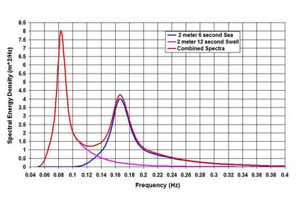 In this piece let us attempt to see more of the Ocean Waves – the spectrum – and how to describe it. The wind generated ocean waves are described by many names – Sea State (sea surface undulations in a storm area) – Random Waves (waves with no apparent systematic pattern) – Irregular Waves (waves with no easily identifiable wave form). The relevance of the last two terms becomes evident when one examines a wave train individually – wave-by-wave. But with the introduction of the signal processing routine – the Fast Fourier Transform (FFT) since 1965 (J. W. Cooley and J. W. Tukey), and its application in digital processing has led to efficiency in wave studies – yielding a new term and meaning – and this term is Spectral Waves. Let us try to see what it means.
Again, literature is full of materials on the subject but perhaps the Coastal Engineering Manual (CEM) of USACE (United States Army Corps of Engineers) is adequate for most purposes. Parts of this piece will also be based on three of my publications:
Before going into discussing the Spectral Waves, it may be helpful to spend a little time on the methodology of analyzing Irregular Waves, because it not only has a historical context but is also very insightful in understanding the wave phenomena. If one examines a measured wave time-series, one may feel rather baffled by the data because the expected sinusoidal or symmetric wave is nowhere to be found. The problems then are: how to define the wave height and period, and how to find some meaningful terms from the jungle? It was H.U. Sverdrup and W.H. Munk who answered the questions first in 1947 after World War II. They realized that it was necessary to solve a technicality first – should the wave height be measured from the trough to the following crest or from the crest to the following trough? The first approach is known as the zero-downcrossing method (starting from the point where water level starts crossing the still water line downward), and the second as the zero-upcrossing method. Because of the irregularity, the two methods do not yield identical results individually, but in aggregate, for let us say 1000 waves; both the methods yield nearly the same results. The authors have also realized that the mean wave height of the group may underestimate the group’s energy and effective forces. Therefore they have defined a very important parameter that continues to shape the meaning of the wave group in coastal engineering. This parameter is known as the significant wave height, Hs or H_1/3 – the average of the highest one-third of the wave group. Another important characteristic was observed by M.S. Longuet-Higgins in 1952. He found out that the frequency distributions followed certain patterns – the water levels as Gaussian Distribution (a symmetric distribution about the mean), and the wave heights as the Rayleigh (named after British physicist John William Strutt known as Lord Rayleigh, 1842 -1919) Distribution. The latter is a skewed distribution where the mean, median and mode do not coincide. The fitting to a known distribution was good news because it allowed scientists and engineers to define some useful parameters. For example, in a situation where 1000 waves are considered, if Hs = 1.0 meter, the maximum is 1.88 meter, the mean is 0.63 meter. Two more parameters are also important – the root-mean-square, Hrms = 0.71 meter often used for estimating sand transport; and the average of the highest 10th percentile, H_1/10 = 1.27 meter often used for determining wave forces on structures. How about the wave period distribution? The answer to the question by M.S. Longuet-Higgins in 1962 showed that wave periods followed Gaussian Distribution. However in 1969 C.L. Bretschneider showed that the squares of the period followed Rayleigh Distribution. The problem was further refined by S.K. Chakrabarti and R.P. Cooley in 1977. Let us try to see it more when discussing the wave spectra. One more thing before we move on to discussing the Spectral Waves. We have tried to see in the Duality and Multiplicity in Nature and Ocean Waves pieces on the NATURE page, and in the Transformation of Waves piece on the SCIENCE & TECHNOLOGY page that most natural waves are spectromatic and asymmetric starting from the time they are born. The closest approximation to the monochromatic and symmetric waves is the deep-water swells that have traveled from the storm area far into tranquil sea water. One experiences long crested (crest is relatively long perpendicular to the direction of wave propagation) swells in the sea where there are no winds to cause them. . . . How a long wave like tide is described in spectral terms? Tidal analyses and predictions are mostly based on spectral decomposition and superposition. The processes of decomposition by Fourier (French mathematician and physicist Jean-Baptiste Joseph Fourier, 1768 – 1830) and Harmonic analyses allow scientists to resolve the tidal wave to find the amplitude and phase of the contributing frequencies – those responsible for generation – as well as those developed by nonlinear interactions within the basin (e.g. my 1991 COPEDEC-PIANC paper: Tidal observations and spectral analyses of water level data in the mouth of the Ganges-Brahmaputra-Meghna river system). The decomposed parameters are then superimposed to predict tide by taking account of the constituent speed, annual nodal factor, astronomical argument etc. If presented as a spectrograph, it can be seen that most of the tidal energy is concentrated in the Semi-diurnal Principal Lunar Constituent. The reason for highlighting the spectral treatment of tide is to show the difference of it from the spectral description of wind waves. In the spectral treatment of wind waves, individual waves are not resolved and decomposed (although they can be analyzed as such like the Boussinesq modeling, Joseph Valentin Boussinesq, 1842 – 1929) to identify wave phases like tidal analysis. Instead time-series water surface elevations about a datum (such as the Still Water Level) are treated as signals by subjecting them to FFT analysis to translate the time-series into the frequency series of elevation variance – the energy density. While doing so, a cut-off frequency or Nyquist (Harry Nyquist, Swedish-American electronic engineer, 1889-1976) frequency is defined to indicate that the measured water levels cannot be resolved below twice the sampling interval. This treatment of water levels as a function of frequency is a simplification of the true nature of ocean waves – and is termed as one-dimensional spectrum. In reality ocean waves are also a function of direction – giving rise to the term directional spectrum (e.g. L.H. Holthuijsen in 1983). What we have discussed so far is the analysis of measured waves depicted in a spectrograph. How to model it to be useful for forecast? Many measured spectra hardly follow a definite pattern, but that did not stop investigators to model them. They proposed the so-called parametric empirical models to best describe the measured spectrum. Because of this approach, a certain model may not be representative for all water areas. Let me outline some of them briefly in this piece, I intend to talk more about them in the SCIENCE & TECHNOLOGY page at some other time. . . . As a forecasting tool, most of the models relate the spectrum to the wind speed, fetch (the distance along the wind direction from the shore to the point of interest) and storm duration (the duration of storm with a relatively unchanged sustained wind speed). Perhaps the 2-parameter spectrum proposed by C.L. Bretschneider in a paper in 1959 was the first of its kind. The paper by W.J. Pierson and L. Moskowitz in 1964 set the stage for describing the single-parameter wave spectrum for a fully developed sea state. In 1973, a 5-parameter spectrum known as JONSWAP (Joint North Sea Wave Project) spectrum was proposed by Hasselmann and others. It became popular as a forecasting tool for fetch-limited (when the storm duration is higher than a threshold that depends on the wind speed and fetch) conditions. Most of the proposed spectra are single peaked, which means if a wave field represents both wind waves and swells, the representation will not be accurate. In the single-peaked spectrum, the peak frequency or reciprocally the peak period Tp is defined as the period of the highest wave energy of the spectrum. On the question of double peaks, M.K. Ochi and E.N. Hubble came to the rescue in 1976 by proposing a 6-parameter spectrum that could describe both wind wave and swell spectra. To illustrate the nature, I have included an image of JONSWAP spectra – for peaks representing a 6-second (0.17 Hertz) sea and a 12-second (0.08 Hertz) swell, and the combined spectrum. Now that we have defined Tp and have some ideas about the wave period distribution, let us attempt to see how different wave periods in the distribution relate to each other. Again for about 1000 waves, if the Tp is 10 second, the zero-upcrossing period is 7.1 second, the significant wave period is 9.5 second, and the mean wave period is 7.7 second. Well so far so good, and I like to leave it at this for now. Sorry that the piece is steeped with technical terms and references – but unfortunately that is how the topic is. Yet many more investigators deserve credit but could not be highlighted in this short piece. Many of the proposed spectra are reviewed by Goda (Yoshima Goda, 1935 – 2012) in 2000, and also briefly in my Encyclopedia article in 2005 (the 2017 update). Before finishing, I like to touch upon three more aspects – the relation between Hs and the spectral determination of this parameter, the relationship between wave height and period, and the spectral evolution of waves. The significant wave height in a spectral approach, symbolized as Hmo or the zero-th moment is determined as 4 times the square root of the area under the spectrum. It turns out Hs and Hmo are not identical in shallow water, as well as in the cases of long-period waves. In both the cases Hs registers higher value than Hmo. . . . The relationship between wave height and wave period is not unique – which means that a wave of the same height could exist both in high and low periods, or as a rephrase a wave of the same period could exist both in high and low heights. It becomes clear when one develops a joint frequency scatter of wave heights and periods. It turns out that a relationship could be established if one takes account of the wave steepness (ratio between wave height and local wave length). In my 2015 paper, I have proposed a relation that shows the wave period as a function of the square root of the wave height and reciprocal of the wave steepness. How does a wind generated wave-spectrum evolve over time as it propagates? I have addressed the question somewhat in the Transformation of Waves piece. Apart from the dispersion and separation of the long-period waves from the group, spectral evolution occurs through the wave to wave interactions. In deep-water, the evolution process known as the Quadruplet, accounts for spreading out the energy in both ways – towards the higher and lower frequencies, and also in directions (which means that the spectral peakedness flattens out). While spreading out of the peak energy occurs in deep-water, in the shallow refraction zone the wave to wave interactions result in a one way process known as the Triad – the transfer of the peak energy to the high frequencies (or low periods). Perhaps this process results in a spectral evolution that approaches the specter of a solitary monochromatic wave in very shallow water. . . . . . - by Dr. Dilip K. Barua, 27 October 2016
After the piece on Linear Waves, it only makes sense that I start this piece talking about Nonlinear Waves – from symmetry to asymmetry – from the processes of a zero residual to the complicacy of residuals. The nonlinearity is the characteristic signature of shallow water waves – and is also a recognizable feature of spectral wind waves that go through the nonlinear processes of interactions and high steepness. We have identified in earlier pieces that the single most important parameter, the Ursell Number, U = HL^2/d^3 (H is wave height, L is local wave length and d is local water depth) characterizes a wave as asymmetric or nonlinear, when U is greater than 5.0. The Ursell Number is universally applicable to all oscillatory flows, whether they are a short wave (like wind wave and swell) or a long wave (like tsunami, storm surge and tide).
Some of the materials covered in this piece on tidal nonlinearity are taken from my Ph.D. Dissertation (Dynamics of Coastal Circulation and Sediment Transport in the Coastal Ocean off the Ganges-Brahmaputra River Mouth, the University of South Carolina, 1992) along with two of my relevant publications:
Many investigators are credited with developing the nonlinear wave theories. To name some, perhaps we can start with Stokes (British mathematician George Gabriel Stokes, 1819 – 1903; Stokes Finite Amplitude Wave Theory), J. S. Russell and J. McCowan (Solitary Wave Theory), D. J. Korteweg and D. de Vries (Cnoidal Wave Theory), Robert G. Dean (Stream Function Theory) and J. D. Fenton (Fourier Series Theory). Many more investigators were involved in expanding and refining the theories, some names include R. L. Weigel, L. Skjelbreia, R. A. Dalrymple and J. R. Chaplin. . . . With this brief introduction, let us now try to understand what nonlinearity means exactly. To illustrate it, I have included two images showing the wave profile, surface horizontal orbital velocity and acceleration for the same 1 meter high 8 second wave, I have shown in the Linear Waves piece. Depicting the parameters for half the wave length, it is immediately clear how the crest is heightened and the trough is flattened when the wave propagates straight shoreward from U = 5.0 to 22.6 (note that 22.6 is near the threshold at which waves can also be treated as Cnoidal). Horizontal water particle velocity has nearly doubled at the crest with the reduction at the trough. For acceleration, the change is not only in the increase in magnitude but also in the phase shift from the symmetry at quarter wave length to the forward skewed distribution. Even this nonlinearity as complicated as it is – is a simplification of the reality because more processes such as reflection and interactions play a role in defining the wave evolution in the nearshore region. We have talked about Stokes Drift in the Transformation of Waves piece on the SCIENCE & TECHNOLOGY page. Stokes Drift or mass transport horizontal velocity represents a nonlinear residual in the direction of wave propagation, and is about one order less in magnitude than the horizontal orbital velocity. For the nonlinear wave at U = 22.6, while the peak surface horizontal orbital velocity is 0.96 meter per second, the drift is roughly about 5 centimeter per second. This drift may seem very small, but a particle traveling at this speed will travel to 180 meter in an hour. Before going further, an important parameter – the local wave length L needs some attention. We have seen in the Linear Waves piece that determining L iteratively has become easy with the modern computing systems, or by applying the Hunt (H. N. Hunt, 1979) method. However as waves become nonlinear, the wave length starts to deviate from the L determined by Linear Wave Theory. It turns out that at U > 5.0, the deviation becomes increasingly larger as U increases, but remains within about 10%. Why understanding the nonlinear wave phenomenon is important? A simple answer to the question is that the nonlinearity of oscillatory flows is responsible for many processes that define a coastal system behavior and characteristics, and in the behaviors of hydrodynamic loading on, and stability of in-water and waterfront structures. Let me try to outline three of them briefly. . . . The first is the effects of the increase and phase-shift of the orbital velocity and acceleration as shown in the images. These processes have significant implications for wave-induced drag, lift and inertial Morison forces (J. R. Morison and others, 1950; forces on slender members) on coastal and port structures. Horizontal drag and inertial forces are relevant in terms of the maximums; therefore as the maximums increase so do the forces. When I stated about the phase-shifts and the relevance of maximums, did anyone notice a contradiction in my statement of Morison forces? Well there is one – the contradiction is due to one of the methods engineers often apply to accommodate some maximums – however unscientific the method may appear – for a conservative and safe design by implanting the so-called Hidden Factor of Safety. Let us discuss more of this aspect in the SCIENCE & TECHNOLOGY page along with my ISOPE paper (Wave Loads on Piles – Spectral Versus Monochromatic Approach, 2008). . . . How does one define the increased nonlinear maximums in terms of asymmetry? Some of my works (not published) indicate that one could relate the amplitude asymmetry of velocity and acceleration in terms of U. Once such a relation is established, it becomes rather easy to determine the nonlinear Morison forces. The second is the effect of the nonlinearity as it interacts with the seabed – the processes generate enhanced turbulence, and when the threshold is exceeded, they are responsible for erosion and resuspension of sediments. Depending on circumstances, nonlinearity is responsible for residual transports toward the onshore, offshore or longshore directions. How to characterize the residuals? I will try to answer this question based on my Ph.D. works and the two relevant publications already mentioned. This will be done for tide, tidal currents and Suspended Sediment (mostly fine sediments that are kept in suspension in the water column by currents and turbulence) Concentrations (SSC). One method to indicate the residuals e.g. of to-and-fro tidal currents (currents are vector kinematics with both magnitude and direction) is to make vector addition of the individual measurements (such as hourly) – such a method immediately shows that a circle cannot be completed because of nonlinearity – and also due to the effects of other superimposed currents such as a river discharge or wind drift, if present. If seaward currents are high at river mouths, residuals are mostly seaward; on the other hand, in absence of a river current or wind drift, tidal asymmetry is responsible for landward transport, and accumulation of fine sediments in tidal flats. These effects of varying superimposed currents and asymmetries often stratify a shallow and wide coastal system horizontally – the coastal ocean off the Ganges-Brahmaputra system is one of such systems. The residual current vectors are a good indicator of, and to where suspended fine (mostly silt and clay sized particles) sediments or water-borne contaminants are likely to end up. The combined tidal current and SSC measurements over time and over the depth can be analyzed applying a procedure known as the linear perturbation principle – a method of vector averaging and identifications of perturbations from the mean. The procedure yields some 5 terms accounting for non-tidal actions, and for the asymmetries of tide, tidal currents and the hysteresis of SSC over time and over the depth. Such methods of separating the components are very useful to provide valuable insights into the identification of processes responsible for certain actions and behaviors. The third is on the most dynamic region of wave action – the surf zone. This is the region where the wave nonlinearity reaches its ultimate stage by breaking as the horizontal wave orbital velocity overtakes the celerity. The breaker line or rather the breaker zone is not fixed, because the breaking depth together with the effects of rising and falling tides is related to the changing wave height. The transformation of the near-oscillatory waves into the near-translatory water motion by wave breaking and energy dissipation is the most recognizable process in this zone. Let us try to see more of it at some other time. . . . . . - by Dr. Dilip K. Barua, 20 October 2016 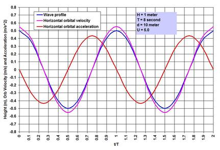 Let me begin by saying that linear waves rarely exist in a natural ocean wave environment, yet the simplification and approximation applied to treat waves as such are very useful for many purposes. These purposes are well served especially for cases in deep-water conditions (where the local depth is greater than half of the local wave length). The simplified and approximated wave is known variously as Linear Wave, Small Amplitude Wave, 1st Order Wave or Airy Wave in honor of George Biddell Airy (1801 – 1892), who was attributed to have derived it first. All natural water waves are gravitational waves – not in a sense that they are generated by gravity, but rather by the fact that gravity is the restoring force – in an equilibrium process between the disturbing and restoring forces.
Literature is full of materials dealing with the Linear Wave Theory. Perhaps the Coastal Engineering Manual (CEM) series produced by USACE is adequate to satisfy many curiosities about ocean waves. In the Ocean Waves piece on this page, and in the Transformation of Waves blog on the SCIENCE & TECHNOLOGY page we have talked about the nature of ocean waves and the transformation processes in plain and poetic terms. Before going further into discussing more of the wave aspects, perhaps it is necessary to introduce the simplicity of linear waves first. Let me try to do that in this piece. What are the approximations and simplifications applied to derive it? A linear wave is nothing but the representation of a circle – in the symmetry of a sinusoidal or harmonic wave. This is obtained by Airy solving the unsteady Bernoulli (Daniel Bernoulli, 1700 – 1782) equation to the 1st order. His solution is based on four major assumptions, that the wave motion is: (1) irrotational (no shearing between layers of motion), (2) progressive (continuous in motion in the direction of propagation without reflection), (3) very small in amplitude compared to the length of the wave, and (4) the motion is 2-dimensional confined within a slice of water cut to the depth along its length of propagation. When the first three assumptions are invalid, the wave loses its symmetry and a nonlinear wave theory applies. . . . What are the fundamental characteristics of a linear wave? From previous discussions we have learned that a wave can be described by 3 fundamental parameters: wave height H (the height from trough to crest), local wave length L or wave period T (measured simply from crest to crest), and the local still water depth d. As we have seen earlier, a very useful parameter proposed by Fritz Joseph Ursell (1923 – 2012) uses these three parameters to indicate whether waves can be approximated by the 1st order processes of the Linear Wave Theory. This parameter known as the Ursell Number describes a threshold combining the two ratios H/d and d/L, and is given by U = HL^2/d^3. It turns out that for all practical purposes, waves can be assumed to be symmetric or linear, when U is equal to or less than 5.0. In addition, two more parameters appear in all the terms describing the wave properties in time and space. The first, useful to describe the wave in time, is known as the wave angular frequency and is given as a ratio between 2*pi and T. The second, useful to describe the wave in space, is known as the wave number and is given as a ratio between 2*pi and L. The Greek symbol pi is a universal constant defining a circle and represents the ratio between the circle perimeter and diameter. The wave length L is a unique function of T in deep water, but in shallower water it becomes dependent on depth d as well. Except in very shallow water, it becomes rather cumbersome to determine the local wave length because L appears on both sides of the equation. The past coastal engineering literature had elaborate graphical methods to facilitate local wave length computations. But with the arrival of digital computation, iteration has become easy to determine it exactly. However a simple method proposed by Hunt in 1979 is incredibly accurate very close to the exact iterative solution. . . . Let us try to chalk out some of the salient linear wave characteristics in order to understand the simplicity of it better. To help us in this regard, I have included an image showing the wave profile and surface wave kinematics for a 1 meter high 8 second wave in 10 meter of water depth. The horizontal axis of this image is time normalized by the wave period.
We have talked about external energies generating waves and propelling them to the destiny of transporting the gained energy forward. How much energy does a wave carry? What is its power? One simple way to answer these questions is by the Linear Wave Theory. Like all waters in motion, energy can be separated into two components – the potential energy and the kinetic energy. Potential energy is due to the displacement of water mass above still water level (SWL), and the kinetic energy is due to the water particle velocity. It turns out that the two components of the wave energy are equal to each other, and are proportional to H^2. This means that the energies of 1 and 2 meter high waves vary by 1 to 4. Wave energy is generally quoted as energy density, which refers to the energy per unit wave length. This means that a wave of the same height carries more total energy for a long period wave than a shorter one. The power is a vector term that works in the direction of wave propagation. Wave power is the product of energy density and celerity (or group celerity for a spectral wave). The wave power is also known as wave energy flux or wave action. The method of balancing the wave action lets one to determine the transformed and/or transmitted waves across varying depths or in situations of wave-structure interactions. . . . There are two other important terms that require some attention – these are known as the radiation stress and momentum flux. Both of these horizontal forces in the direction of wave propagation are caused by the dynamic pressure and the pressure exerted by kinetic energy (also dynamic in nature). Radiation stress develops due to the excess pressure – and is due to wave nonlinearity. Let us talk about this some other time. Dynamic Pressure is the result of changing water surface elevation up and down of SWL – and is in phase with wave profile. What does this imply? The dynamic pressure implies that one feels excess pressure (compared to hydrostatic pressure) when under the wave crest and less or an uplift pressure under the trough. This process allows scientists to measure wave height by deploying subsurface pressure sensors. The concept of momentum flux has been proposed by Steven Hughes of USACE in 2003. The instantaneous value of this parameter is the summation of the horizontal dynamic pressure and the pressure induced by the kinetic energy. Among others, the momentum flux is very useful to assess wave interactions with intervening structures and depth changes. Well, these are some of the important aspects of linear waves in a nutshell. Let us finish this piece with a quote from Einstein (1879 – 1955): everything should be made as simple as possible, but no simpler. . . . Here is an anecdote to ponder: In the meantime the disciple went on a vacation – fully paid. The poor master also went on a vacation – but unpaid, and just in the neighborhood listening to the songs of life and Nature. . . . . . - by Dr. Dilip K. Barua, 13 October 2016  I have chosen the title of this piece to describe the deltas created by rivers such as the Amazon, the Nile, the Mississippi and the Ganges-Brahmaputra-Meghna (GBM) river systems, each of which debouches into the coastal ocean. The purpose is to distinguish this type of delta from its cousins – the land deltas such as the Okavango Delta in Botswana, the lake deltas, and flood and ebb tidal deltas we see at coastal inlets along alluvial shores.
All deltas have one common feature though. Deltas are a net sediment depositional geomorphic area, and are built when the sediment carrying capacity of a constricted flow is lost in relatively wide open water. They are the typical planform areas where a flow forks outward into multiple distributary channels, cut through the fresh deposits of shoals and islands. Large river deltas are important for at least two important reasons. The first is their capacities to support many unique aquatic creatures, and flora and fauna that call deltas their homes. The second is the delta processes that bury dying plants and creatures. Through geologic time, this second process is responsible for accumulation and trapping of hydrocarbons released by decaying lives in sedimentary basins. . . . A delta is the topic of studies by at least four different disciplines of physical and applied sciences. There are the geologists in search of finding the clues to understand ancient deltaic hydrocarbon deposits – in attempts to connect the present to the past; and the geographers in search of characterizing the patterns of processes – the present and the past. The oceanographers primarily focus on hydrodynamics with some attentions paid to sediments as far as the bed-resistance to flow is concerned. In the process they discover and propose many easily understandable behavioral models coining and defining different terms to describe a delta. They mainly conduct field works far and wide, and with supporting laboratory experiments, try to connect dots to help us understand the delta processes better – not only with the behavioral models but also with the continuing progress on process-based models. The first two of the above disciplines delve into the long scales of space and time, while the oceanographers mainly focus on contemporaneous processes. The applied scientists or civil/hydraulic engineers primarily concentrate on short engineering time-scale in the order of 100 years or less. Standing on the foundations created by geologists, geographers and oceanographers, but with the safety, stability and effects of structures/interventions in mind, engineers’ methods are mostly based on investigations and scale modeling to derive process-based models in the controlled and manageable conditions of a laboratory. Supported by field works, they focus on hydrodynamics as well as on the processes of sediment transport and morphology. While the above generalizations and differences hold in general, there are considerable overlaps among the disciplines cross-fertilizing one another. This is especially true in advanced studies – where it is difficult to distinguish a certain work belonging to one discipline or the other, if the authors’ affiliations are not revealed. My professional involvement with studying coastal dynamics in a deltaic environment started with my works at the Land Reclamation Project – a Dutch project in the GBM coastal delta of Bangladesh – tasked to develop engineering plans to promote accretion, and for reclamation of the new delta landmasses. The involvement led to my Masters degree in coastal/hydraulic engineering at the UNESCO-IHE, Delft, the Netherlands; and later to my Ph.D. at the University of South Carolina (USC). Some of my works are published in journal and conference proceeding titles like, Elsevier, Taylor & Francis, Springer, Journal of Coastal Research (JCR), American Shore and Beach Preservation Association (ASBPA) and American Society of Civil Engineers (ASCE). The USC academic program gave me the opportunity to participate in a field trip to have a bird’s eye view by flying over the unique form of the Mississippi Delta. . . . With this little background, let us now try to have a glimpse of the processes that lead to the formation of deltas at a coastal river mouth. Some of the materials I will cover are taken from one of my discussion articles {Discussion of ‘Development and Geometric Similarity of Alluvial Deltas’, ASCE Journal of Hydraulic Engineering, 2002}. From the perspectives of delta building, two distinct processes can be identified at the very outset – these are the relative magnitudes of constructive and the destructive processes. Let us first try to see them by highlighting some examples. One can say that the ideal or the most recognizable delta morphology of the Mississippi and the Nile rivers shows more of constructive influences than the less recognizable delta of the GBM system. The Mississippi and the Nile flows face very low tidal forcings from the Gulf of Mexico and the Mediterranean Sea, respectively. However, since the commissioning of the Aswan Dam in July 1970, and because of several works on the Mississippi River basin (see the 2012 USGS report: A Brief History and Summary of the Effects of River Engineering Dams on the Mississippi River System and Delta), the delta morphologies of these two rivers have been increasingly getting more exposed to the destructive processes than the constructive ones. Although I have mentioned these two examples, all the major river systems and their deltas have been getting affected by increasing interventions – like the Farakka Barrage constructed on the Ganges River in 1975. . . . What are the constructive and destructive forces exactly? First let us try to see the types of the constructive processes. In simple terms these are the amount of sediment loads per a unit volume of flowing water, and the type of sediments a river transports – the larger the sediment load, the higher is its chance of forming a delta. And the rivers carrying higher percentage of sand than the fine fractions of silt and clay contribute more to the delta building processes. The destructive processes are the adverse ambient coastal environments, within which a river debouches – the submarine topography, tide, wave, and most importantly the episodic events such as tectonic activity, flood and storm surge. When a river debouches at a steep coast or a submarine canyon, the chances are that the river will only be able to build a submarine delta. A submarine delta or fan develops quietly without the disturbing effects of tide, wave and storm surge. The half-day oscillating tidal forcing erodes and resuspends the river-deposited sediments and transports them back and forth. The tidal processes align the sand shoals and islets with the prevailing current direction, and winnow the sediments to make the residual transport of the fines in preferential landward directions. The GBM delta is the typical example of a tide-dominated delta. Pounding waves work in a similar fashion in time scales in the order of 10 seconds – they winnow the deposits and transport the sand fraction in cross-shore and downdrift longshore directions to form depositional features like barrier islands. But the least understood episodes of tectonics, river flood and storm surge affect the delta evolution, perhaps more than any other. Tectonic uplift or subsidence either in secular trend or in episodes, shifts the epicenter of the delta deposits from one location to another – in the process, flow-shares of distributaries are changed. And the effects of flood? Let us try to see them. When a distributary becomes too long, its flow becomes sluggish [the Common Sense Hydraulics piece on the SCIENCE & TECHNOLOGY page indicates how delta progradation causes reduction of flow velocity], and the river looks for opportunities to find a steeper slope to the sea. A river flood comes with the help, and when the conditions are right, it cuts through the shoals or moribund channels giving a new life to the delta flow-distribution dynamics. Similar episodes happen when a storm surge forcing occurs on a delta landscape. Its power can erode and sweep away sand deposits out to the sea or could cut new channels redefining the delta dynamics. The historic Mississippi delta sequence during a portion of the Holocene Transgression period, shown in the image (credit: anon) gives an impression how deltas change their depo-centers over time. Similar shift happened in the GBM delta when the Ganges River shifted to the east to meet the Brahmaputra and the Meghna rivers, to reach out to the sea as a combined flow. . . . Delta building processes go through three major hydraulic phases – the first two primarily represent the sequences of constructive forces, but the third phase is a vigorous showcase of interactions between the constructive and destructive forces. The first phase processes are better understood through a jet theory. This theory in simple terms, explains how a jet emanating from a river, a diffuser outlet or a ship propeller, expands into the wide-open water. The expansion decelerates the flow velocity, and the river has no option other than to depositing its sediment load – the coarser fraction within the immediate vicinity, and the finer fractions further into the sea. Geologists have termed the depositional features as the seaward bottomset bed of the fines, and the coarse deposits of the topset bed. Like the submarine delta, the bottomset bed develops quietly with minimal disturbance from tide and wave. An episodic storm surge may affect the bottomset processes to some extent though. The topset bed or the delta proper, progrades forward into the sea through the avalanching of sand on the inclined foreset bed. In some instances when the foreset delta front becomes too steep, a sudden rapid submarine slope failure occurs causing tsunami. There are many examples of this type of tsunamis; some are often triggered by tectonic activities. Such a tsunami occurred in 1975 – in a little known delta of the Kitimat Arm at the head of the Douglas Channel fjord in British Columbia. The second phase occurs when the decelerated jet faces further frictional resistance from the built-up deposits of the topset bed. The result is the erratic channel and depositional patterns occurring in lateral expansions. Scientists try to understand this phase by describing and formulating the processes mostly through behavioral morphometric models. The third phase represents the most complex processes of delta evolution through time, showcasing the intensive actions and reactions of constructive and destructive forces. In this phase, delta deposits have already anchored themselves through colonization by plants and trees – therefore flows encounter more resistance. The destructive forces of tide and wave, and the episodes of extreme events when dominant, can completely redefine the delta planform evolution. Understanding delta dynamics as complicated as they are, has been made much easier with increasing applications of numerical computational models – by the advanced models dynamically coupling hydrodynamics, wave mechanics and sediment-morphology modules. Let us try to talk about this important topic at some other time. . . . Here is an anecdote to ponder: The disciple asked the master, “Sir, what do the delta processes tell us?” The master smiled, “Umm! Let me see. A river matures on its journey to the sea overcoming resistances and obstacles, meeting something different and overwhelming in the end. The loads it carries on its shoulder appear burdensome. It finds the comfort to be in right place to unload to build something new – the delta. Now, you figure out what it says to life and social living of humans.” . . . . . - by Dr. Dilip K. Barua, 15 September 2016 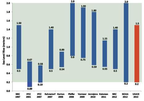 The changing climate (In a later article Warming Climate and Entropy, posted in December 2019 – I have tried to throw some lights on the climate change processes of the interactive Fluid, Solid and Life Systems on Earth – the past, the present and the future) with its consequent effect on sea level is the most du jour topic of our time. It is not surprising – because there are many reasons for such popular attentions and human concerns. Some two-thirds of world’s seven billion people live within 100 miles of the coastline with the economic activities ranging from recreation to exploitation of sea resources to waterfront living, to gateways catering trade and commerce through many port and harbor infrastructure.
. . . There is a caveat however – that we should watch ourselves not to lose the voice of reason by yielding in to the mob mentality of bullying and accepting whatever floats around. The fluctuation of sea level with the consequent transgression and regression of the shoreline is a complex phenomenon – and as we will try to have a glimpse – it would appear that it is a complicated response to many forcings of various scales and magnitudes – both terrestrial and extra-terrestrial. In this piece I will mainly focus on the science of sea level rise (SLR), and intend to cover the consequences and adaptive responses to SLR on the SCIENCE & TECHNOLOGY page at some other time. During the past four decades considerable amounts of works have been conducted by multiple national and international organizations on SLR and implications. It is only possible to have a glimpse of it in this piece. My discussions are primarily based on knowledge gleaned from such resources as: UN entity IPCC (Intergovernmental Panel on Climate Change), US CCSP (Climate Change Science Program), US NOAA (National Oceanic and Atmospheric Administration), US NRC (National Research Council), US EPA (Environmental Protection Agency), USGS (United States Geological Survey), USACE (United States Army Corps of Engineers) and the Canadian National Research Council (CNRC). Some of the US works are published by the National Academies Press (NAP). To give a little background, I got interested in SLR in the 1990s, not so much as part of my professional responsibilities at that time, but as an effort of self-educating myself. The effort resulted in an article I published in 1990 in a Bangladesh national weekly. The article must have caught attention of some, because it was translated to Bengali subsequently. The concern about the effects of SLR on Bangladesh has begun to get global attention because most of the country’s territories are low lying deltaic coastal landscape. Dutch Government initiated some of the studies, and I was fortunate to officially review some of their projects. I was also involved in another project in vulnerability assessments of SLR. Some other subsequent involvements in USA and Canada were mostly in the scopes of side-line responsibilities. . . . Perhaps it is helpful to know a little bit of geologic history to understand the phenomenon of SLR. Long-term studies of scientific data indicate that the present sea level, stands on the geologic interglacial period, perhaps at its peak. Geologic history tells us that there have been four major cycles of glacial-interglacial periods with the corresponding low and high sea level stands in the 400,000 years before present (BP). The last lowest sea level at -120 meter occurred about 18,000 years BP. Try to imagine the scenario of that time when our shoreline was at the edge of the present continental shelf. During that time many landmasses separated by shallow seas were connected together. We still see the remnants of the past shoreline as river mouth scars or submarine canyons. What are the causes of these past sea level fluctuations? As pointed out, these fluctuations in sea level are due to many glacial and interglacial periods, or ice age sequences. Scientists have identified some eight causes for ice age sequences: (1) change in the Earth’s atmosphere or climate; (2) relative positions of the continents or change in the volumes of ocean basins; (3) fluctuations of ocean currents; (4) uplift of the roof of the world – the Tibetan Plateau; (5) variations in Earth’s orbit (known as Milankovitch Cycles); (6) variations in Sun’s energy radiation; (7) volcanisms; and (8) fluctuations in dust-ice albedo. So the real reasons for sea level fluctuations are much more complex than we tend to think. They vary from extra-terrestrial factors to the Earth’s atmospheric, topographic and oceanic controls, to volcanism and albedo change. . . . Now let us try to attempt to look at its behavior in the recent geologic past. From 18,000 years BP sea level has been rising – but not at a constant rate, rather at variable rates – sometimes faster than other times. This process is known as Flandarian Transgression or Holocene Transgression. On average, the SLR rate slowed down onward from 5000 years BP when the sea level stand was at –10 meter. We can generalize the rates in orders of magnitude like this: from 18,000 to 5,000 years BP, SLR rate was on average +10.0 millimeter per year, and the slowed rate from 5,000 years BP was about +1.5 millimeter per year. Well, if SLR rate has really slowed down to such an extent, why should there be so much concern? The answers to the question can be found in at least three important considerations. First, humans have encroached into the domain of sea at an alarming manner. Therefore, our SLR tolerance threshold has very little room for accommodation. We have built coastal cities, human habitation and port infrastructure by advancing into the sea redefining the shoreline. Scientists had very little idea about the phenomenon of sea level fluctuations until recent time – therefore they were not in a position to warn of the consequences of our appetite and adventure for more of the sea; even if they did, it fell into deaf ears of the decision makers. The second is the narrow window of tolerance within which all plants and living creatures including humans can survive. As we have seen in the Natural Equilibrium blog on this page, system of things remains in a state of delicate balance in Nature, in quests to attain dynamic equilibrium. The narrow tolerance threshold of humans and other flora and fauna means that they cannot afford to live when the adaptation or equilibrium time is long. In addition, the narrow tolerance levels make life and habitat vulnerable to the effects of rather minor changes. Because of the complexity of processes, these effects in stresses and disruptions of normal ways of lives and livelihoods are not always easy to address. The third, and perhaps the most important one is the disturbing findings of scientists that the recent SLR rate is highly correlated with global Warming Climate change. If one breaks down the recent past, within the past 1000 years CE, SLR rate was 0.0 millimeter per year, after that the rate rose to +0.6 millimeter per year, then declined to -0.1 millimeter per year for a short period of time. Starting roughly at the middle of the 20th century, the SLR rate has been rising at +2.1 millimeter per year. Scientists have found that this accelerated rate is positively correlated with the increasing greenhouse gas emissions, rise in atmospheric, land and oceanic temperatures, and the retreats of glaciers in the Polar Regions. The conclusion is that human activities are responsible for such an accelerated rate, and scientists have coined a new term, the Anthropocene Epoch starting in 1950 to mark the human footprints on the environment. . . . So far we have discussed the global SLR rate over time. How about the rates over space? Local SLR rates are highly variable from region to region. Let us try to see how SLR is defined in space. The first is often termed as Eustatic SLR, which refers to global change in the ocean volume – evidently when the basin becomes large, sea level falls, and vice versa. Overall, some other major factors contributing to SLR include: melting of continental and Polar ice masses, reduction in ocean water density and resulting expansion, ocean circulation responsible for distributing the heat and dissolved substances, isostatic rebound of the coastal landmass resulting from melting and regression of glaciers, uplift or subsidence due to tectonic activity, soft sediment consolidation and subsidence, and ocean-atmosphere interaction. Regional uplift or subsidence adds local flavor to SLR - for a subsiding coast SLR is more than an uplifting or rebounding coast. The subsidence can overwhelm the global SLR; for example, at the Mississippi River delta, the present SLR rates vary from +9 to +12 millimeters per year, far higher than the global average. The opposite happens at an uplifting coast. The phenomenon of regional variability - the enhanced SLR on subsiding coasts and the decreased SLR on uplifting coasts - is captured by a new term, the relative SLR. . . . Let us now turn our attention to the most difficult part of the SLR problem – and this is the problem with predicting the future change in sea level. The crust of the problem lies with the predictability of soft models employed by various investigators. We have discussed the typical nature of this modeling problem in the Natural Equilibrium blog on this page as well as in the Water Modeling and Uncertainty and Risk pieces on the SCIENCE & TECHNOLOGY page. To demonstrate it, I have included an image taken from USACE. The USACE has compiled the 2100 SLR predictions conducted by most involved organizations. Looking into the image, two striking feature should attract everybody’s attention. The first is the lack of agreements among the organizations. The second is the large difference between the maximum and minimum of individual predictions. The highest predicted SLR in 2100 is +2.0 m, compared with the lowest prediction of +0.58 m. Accepting one or the other comes with huge environmental risks and financial consequences. One may dare to ask whether the scientific correlation between the SLRs and the global warming is just another anomaly or uncertainty. The chances are that such a suggestion is highly unlikely; even if likely, it is important that humanity tries to minimize its footprint on the environment impacting lives of plants and other creatures. Because an unsustainable approach impacting others has only one door open – that is the door of compromising the future well-being of all. But one thing is sure, that the uncertainties associated with predictions make it hard for decision makers to conceive and develop adaptation strategies. Let us try to address this issue more in the SCIENCE & TECHNOLOGY page at some other time - posted in the Sea Level Rise - the Consequences and Adaptation. . . . Here is an anecdote to ponder: The disciple asked the master, “Sir, because global temperature and sea level stand have changed so many times in the past, I am wondering what would happen if instead of warming, we come across cooling of Earth.” The master looked at him and smiled, “Good Lord, this is not happening in our lifetime! But you have pointed out an important issue – that may haunt humanity at some time in the distant future in the human-scale of thinking. There is no doubt that such a scenario would cause absolute havoc in people’s mind. Perhaps everyone would cry for burning more and more fossil fuels to keep things warm. Or perhaps with lowering of sea level stand with glaciations, people will go further into the sea to build – the human appetite for exploitation will never cease. There may occur a reverse flow of refugees from colder countries to warmer ones – or war may break out.” “Human destiny in the hand of climate change!” “Yes, climate is the ultimate arbiter. Inevitability of such a scenario indicates the necessity of managing the Earth’s resources in a sensible manner for common well-being. The effort of sensible management is no easy task, however – because it would require real commitments from all nations by melting down vicious differences we see now.” “How about artificial creation of energy-emitting sun or suns. I have heard that such high level researches have been sponsored by many countries.” “It is encouraging that this and many other cutting edge researches are being initiated around the world, albeit at a high cost. Scientific leaders are thinking ahead than most of us realize. But practical outcomes of such endeavors usually take very long time – and there are considerable uncertainties in such efforts, even tangible benefits may never materialize. I guess though that the efforts result in gaining and perfection of knowledge in various supporting activities.” . . . . . - by Dr. Dilip K. Barua, 8 Septermber 2016 |
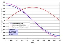
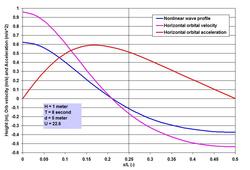

 RSS Feed
